Sunday, March 31, 2019

Reverse Proxy


https://www.linuxbabe.com/it-knowledge/differences-between-forward-proxy-and-reverse-proxy
The main difference between the two is that forward proxy is used by the client such as a web browser whereas reverse proxy is used by the server such as a web server. Forward proxy can reside in the same internal network as the client, or it can be on the Internet.

Forward proxy can be used by the client to bypass firewall restrictions in order to visit websites that are blocked by school, government, company etc. If a website blocked an IP range from visiting the website, then a person in that IP range can use forward proxy to hide the real IP of the client so that person can visit the website and maybe leave some spam comments. However forward proxy might be detected by the website administrator. There are some paid proxy service that has numerous proxy systems around the world so that they can change your IP address every time your visit a new web page and this makes it harder for website administrators to detect.


Reverse proxy is mainly used by server admins to achieve load balancing and high availability. A website may have several web servers behind the reverse proxy. The reverse proxy server takes requests from the Internet and forward these requests to one of the web servers. Most visitors don’t know websites are using reverse proxy because they usually lack the knowledge and tools to detect it or they simply don’t care about it. Nginx can be acting both a web server and a reverse proxy at the same time. HAProxy is another well-known open-source reverse proxy software.


Site Reliability Engineering Book


Chapter 22. Addressing Cascading Failures
If at first you don’t succeed, back off exponentially.
Why do people always forget that you need to add a little jitter?

A cascading failure is a failure that grows over time as a result of positive feedback.1 It can occur when a portion of an overall system fails, increasing the probability that other portions of the system fail. For example, a single replica for a service can fail due to overload, increasing load on remaining replicas and increasing their probability of failing, causing a domino effect that takes down all the replicas for a service.
Causes of Cascading Failures and Designing to Avoid Them
Server Overload
The most common cause of cascading failures is overload. Most cascading failures described here are either directly due to server overload, or due to extensions or variations of this scenario.

Load test the server’s capacity limits, and test the failure mode for overload
This is the most important exercise you should conduct in order to prevent server overload. Unless you test in a realistic environment, it’s very hard to predict exactly which resource will be exhausted and how that resource exhaustion will manifest
Serve degraded results
Serve lower-quality, cheaper-to-compute results to the user. Your strategy here will be service-specific

Instrument the server to reject requests when overloaded
Servers should protect themselves from becoming overloaded and crashing. When overloaded at either the frontend or backend layers, fail early and cheaply.
Instrument higher-level systems to reject requests, rather than overloading servers
Note that because rate limiting often doesn’t take overall service health into account, it may not be able to stop a failure that has already begun. Simple rate-limiting implementations are also likely to leave capacity unused. Rate limiting can be implemented in a number of places:
  • At the reverse proxies, by limiting the volume of requests by criteria such as IP address to mitigate attempted denial-of-service attacks and abusive clients.
  • At the load balancers, by dropping requests when the service enters global overload. Depending on the nature and complexity of the service, this rate limiting can be indiscriminate (“drop all traffic above X requests per second”) or more selective (“drop requests that aren’t from users who have recently interacted with the service” or “drop requests for low-priority operations like background synchronization, but keep serving interactive user sessions”).
  • At individual tasks, to prevent random fluctuations in load balancing from overwhelming the server.
Perform capacity planning
Queue Management
Most thread-per-request servers use a queue in front of a thread pool to handle requests. Requests come in, they sit on a queue, and then threads pick requests off the queue and perform the actual work (whatever actions are required by the server). Usually, if the queue is full, the server will reject new requests.
If the request rate and latency of a given task is constant, there is no reason to queue requests: a constant number of threads should be occupied. Under this idealized scenario, requests will only be queued if the steady state rate of incoming requests exceeds the rate at which the server can process requests, which results in saturation of both the thread pool and the queue.
Queued requests consume memory and increase latency. For example, if the queue size is 10x the number of threads, the time to handle the request on a thread is 100 milliseconds. If the queue is full, then a request will take 1.1 seconds to handle, most of which time is spent on the queue.
For a system with fairly steady traffic over time, it is usually better to have small queue lengths relative to the thread pool size (e.g., 50% or less), which results in the server rejecting requests early when it can’t sustain the rate of incoming requests. For example, Gmail often uses queueless servers, relying instead on failover to other server tasks when the threads are full. On the other end of the spectrum, systems with “bursty” load for which traffic patterns fluctuate drastically may do better with a queue size based on the current number of threads in use, processing time for each request, and the size and frequency of bursts.

Load Shedding and Graceful Degradation

Load shedding drops some proportion of load by dropping traffic as the server approaches overload conditions. The goal is to keep the server from running out of RAM, failing health checks, serving with extremely high latency, or any of the other symptoms associated with overload, while still doing as much useful work as it can.
One straightforward way to shed load is to do per-task throttling based on CPU, memory, or queue length; limiting queue length as discussed in “Queue Management” is a form of this strategy. For example, one effective approach is to return an HTTP 503 (service unavailable) to any incoming request when there are more than a given number of client requests in flight.
Graceful degradation takes the concept of load shedding one step further by reducing the amount of work that needs to be performed. In some applications, it’s possible to significantly decrease the amount of work or time needed by decreasing the quality of responses. For instance, a search application might only search a subset of data stored in an in-memory cache rather than the full on-disk database or use a less-accurate (but faster) ranking algorithm when overloaded.
Graceful degradation shouldn’t trigger very often—usually in cases of a capacity planning failure or unexpected load shift. Keep the system simple and understandable, particularly if it isn’t used often.


### retry
- Limit retries per request
- randomized exponential backoff
- have a server-wide retry budget. For example, only allow 60 retries per minute in a process
- avoid amplifying retries by issuing retries at multiple levels
- Use clear response codes and consider how different failure modes should be handled

MISSING DEADLINES
A common theme in many cascading outages is that servers spend resources handling requests that will exceed their deadlines on the client. As a result, resources are spent while no progress is made: you don’t get credit for late assignments with RPCs.


If handling a request is performed over multiple stages (e.g., there are a few callbacks and RPC calls), the server should check the deadline left at each stage before attempting to perform any more work on the request. For example, if a request is split into parsing, backend request, and processing stages, it may make sense to check that there is enough time left to handle the request before each stage.
DEADLINE PROPAGATION
CANCELLATION PROPAGATION

Slow Startup and Cold Caching
When adding load to a cluster, slowly increase the load. The initially small request rate warms up the cache; once the cache is warm, more traffic can be added. It’s a good idea to ensure that all clusters carry nominal load and that the caches are kept warm


Taming The Long Latency Tail - Handling sloe requests


http://highscalability.com/blog/2012/3/12/google-taming-the-long-latency-tail-when-more-machines-equal.html
Luiz André Barroso, Distinguished Engineer at Google, talks about this fundamental property of scaling systems in his fascinating talk, Warehouse-Scale Computing: Entering the Teenage Decade. Google found the larger the scale the greater the impact of latency variability. When a request is implemented by work done in parallel, as is common with today's service oriented systems, the overall response time is dominated by the long tail distribution of the parallel operations. Every response must have a consistent and low latency or the overall operation response time will be tragically slow. The implication: high performance equals high tolerances, which means your entire system must be designed to exacting standards.
What is forcing a deeper look into latency variability is the advent of interactive real-time computing. Responsiveness becomes key. Good average response times aren't good enough. You simply can't naively scale up techniques to build larger systems. The reason is surprising and has deep implications on how we design service dominated systems:
Google Likes Request Level Parallelism, Which Is Easy

Mom And Apple Pie Techniques For Managing Latency

These techniques the “general good engineering practices” for managing latency:
  • Prioritize request queues and network traffic. Do the most important work first.
  • Reduce head-of-line blocking. Break large requests into a sequence of small requests. This time slices a large request rather than let it block all other requests.
  • Rate limit activity. Drop or delay traffic that exceeds a specified rate. 
  • Defer expensive activity until load is lower.
  • Synchronize disruptions. Regular maintenance and monitoring tasks should not be randomized. Randomization means at any given time there will be slow machines in a computation. Instead, run tasks at the same time so the latency hit is only taken during a small window.

Cross Request Adaptation Strategies

The idea behind these strategies is to examine recent behavior and take action to improve latency of future requests within tens of seconds or minutes. The strategies are:
  • Fine-grained dynamic partitioning. Partition large datasets and computations. Keep more than 1 partition per machine (often 10-100/machine). Partitions make it easy to assign work to machines and react to changing situations as the partitions can be recovered on failure or replicated or moved as needed.
  • Load balancing. Load is shed in few percent increments. Shifting load can be prioritized when the imbalance is severe. Different resource dimensions can be overloaded: memory, disk, or CPU. You can't just look at CPU load because they may all have the same load. Collect distributions of each dimension, make histograms, and try to even out work to machines by looking at std deviations and distributions.
    Different resource dimensions can be overloaded: memory, disk, or CPU. You can't just look at CPU load because they may all have the same load. Collect distributions of each dimension, make histograms, and try to even out work to machines by looking at std deviations and distributions.
  • Selective partitioning. Make more replicas of heavily used items. This works for static or dynamic content. Important documents or Chinese documents, for example, can be replicated to handle greater query loads.
  • Latency-induced probation. When a server is slow to respond it could be because of interference caused by jobs running on the machine. So make a copy of the partition and move it to another machine, still sending shadow copies of the requests to the server. Keep measuring latency and when the latency improves return the partition to service.

Within-Request Adaptation Strategies

The idea behind these strategies is to fix a slow request as it is happening. The strategies are:
  • Canary requests
  • Backup requests with cross-server cancellation
  • Tainted results

Backup Requests With Cross-Server Cancellation

Backup requests are the idea of sending requests out to multiple replicas, but in a particular way. Here’s the example for a read operation for a distributed file system client:
  • send request to first replica
  • wait 2 ms, and send to second replica
  • servers cancel request on other replica when starting read
A request could wait in a queue stuck behind an expensive query or a packet could be dropped, so if a reply is not returned quickly other replicas are tried. Responses come back faster if requests sit in multiple queues.

Cancellation reduces the frequency at which redundant work occurs.

You might think this is just a lot of extra traffic, but remember, the goal is to squeeze down the 99th percentile distribution, so the backup requests, even with what seems like a long wait time really bring down the tail latency and standard deviation. Requests in the 99th percentile take so long that the wait time is short in comparison.

Bigtable, for example, used backup requests after two milliseconds, which dramatically dropped the 99th percentile by 43 percent on an idle system. With a loaded system the reduction was 38 percent with only one percent extra disk seeks. Backups requests with cancellations gives the same distribution as an unloaded cluster.

With these latency tolerance techniques you are taking a loaded cluster with high variability and making it perform like an unloaded cluster.

There are many variations of this strategy. A backup request could be marked with a lower priority so it won't block real work. Send to a third cluster after a longer delay.Wait times could be adjusted so requests are sent when the wait time hits the 90th percentile.

Tainted Results - Proactively Abandon Slow Subsystems

  • Tradeoff completeness for responsiveness. Under load noncritical subcomponents can be dropped out. It’s better, for example, to search a smaller subset of pages or skip spelling corrections than it is to be slow.
  • Do not cache results. You don’t want users to see tainted results.
  • Set cutoffs dynamically based on recent measurements.
http://highscalability.com/blog/2010/11/22/strategy-google-sends-canary-requests-into-the-data-mine.html
Google runs queries against thousands of in-memory index nodes in parallel and then merges the results. One of the interesting problems with this approach, explains Google's Jeff Dean in this lecture at Stanford, is the Query of Death.
A query can cause a program to fail because of bugs or various other issues. This means that a single query can take down an entire cluster of machines, which is not good for availability and response times, as it takes quite a while for thousands of machines to recover. Thus the Query of Death. New queries are always coming into the system and when you are always rolling out new software, it's impossible to completely get rid of the problem.
Two solutions:
  • Test against logs. Google replays a month's worth of logs to see if any of those queries kill anything. That helps, but Queries of Death may still happen.
  • Send a canary request. A request is sent to one machine. If the request succeeds then it will probably succeed on all machines, so go ahead with the query. If the request fails the only one machine is down, no big deal. Now try the request again on another machine to verify that it really is a query of death. If the request fails a certain number of times then the request if rejected and logged for further debugging.


The result is only a few servers are crashed instead of 1000s. This is a pretty clever technique, especially given the combined trends of scale-out and continuous deployment. It could also be a useful strategy for others. 

https://landing.google.com/sre/sre-book/chapters/addressing-cascading-failures/

LogStash Architecture


https://www.tutorialspoint.com/logstash/logstash_internal_architecture.htm

Logstash Service Architecture

Logstash processes logs from different servers and data sources and it behaves as the shipper. The shippers are used to collect the logs and these are installed in every input source. Brokers like Redis, Kafka or RabbitMQare buffers to hold the data for indexers, there may be more than one brokers as failed over instances.
Indexers like Lucene are used to index the logs for better search performance and then the output is stored in Elasticsearch or other output destination. The data in output storage is available for Kibana and other visualization software.
Logstash Service Architecture

Logstash Internal Architecture

The Logstash pipeline consists of three components Input, Filters and Output. The input part is responsible to specify and access the input data source such as the log folder of the Apache Tomcat Server.
Logstash Internal Architecture

https://subscription.packtpub.com/book/big_data_and_business_intelligence/9781787281868/5/ch05lvl1sec31/logstash-architecture
The Logstash event processing pipeline has three stages, they are: Inputs, Filters and Outputs. A Logstash pipeline has two required elements; input, output, and, optionally, filters:
Inputs create events, Filters modify the input events, and Outputs ship them to the destination. Inputs and outputs support codecs which enable you to encode or decode the data as and when it enters or exits the pipeline without having to use a separate filter.
Logstash uses in-memory bounded queues between pipeline stages by default (Input to Filter and Filter to Output) to buffer events. If Logstash terminates unsafely, any events that are stored in memory will be lost. To prevent data loss, you can enable Logstash to persist in-flight events to the disk by making use of persistent queues. 
- send updates to multiple brokers, indexer. 


Linked FollowFeed - (ALT - Aggregator Leaf Tailer)


https://engineering.linkedin.com/blog/2016/03/followfeed--linkedin-s-feed-made-faster-and-smarter
Our existing feed infrastructure, Sensei, suffered from increasing operational costs and it could not perform well with LinkedIn's growth curve in terms of content and members. We needed an infrastructure that could dynamically sieve through the content shared by a member’s network to deliver a list of relevant, ordered, and personalized content while satisfying all requirements of a highly available low-latency application.


Sensei: Previous Feed Infrastructure
  • Sensei: Previous Feed Infrastructure


Sensei, the generic search system built by LinkedIn, which previously powered our feed infrastructure, provided the following features:
  • A distributed, elastic, real-time searchable database built on top of Lucene. This system could be horizontally sharded to cater to an increase in traffic.
  • Built-in support for complex relevance algorithms to rank content records in feed.
Content records were ingested into Sensei’s searcher nodes via Kafka. Queries to Sensei were specified in BQL language, which consisted of both filtering and relevance logic. Requests were received by a broker service which fanned out requests to all searcher nodes. Each searcher node applied some filtering logic to prepare a candidate set for the relevance algorithm. After applying the relevance algorithm, each node returned top N records. Records from all these searcher nodes were aggregated on broker and then sorted according to their relevance scores. Top N records from this sorted list were then returned to the client. As the relevance algorithm is embedded in the query itself, clients could easily A/B test different relevance algorithms.

FollowFeed: New Feed Infrastructure
FollowFeed generates the feed for a member upon request by aggregating content created by entities in which they are interested. An entity can be another member, a company, an educational institution etc. For supporting such complex requests, we need an index that associates content created by an entity with the entity’s unique ID. This index for an entity will be referred to as timeline in this blog post.
A timeline is a chronologically ordered list of records by or about an entity. For example, there are many different records which go in a member’s timeline: member shares an article, member is mentioned in an article, etc. FollowFeed uses this concept of a timeline to compose the feed for the member.
Design Choices
The primary design requirements of the feed infrastructure are:
  • Scalability: Architecture should be easily horizontally scalable for both reads and writes.
  • Read Performance: As this system will support multiple feed use-cases, it’s very important that this system is efficient in terms of read performance.
  • Relevance support: As mentioned earlier, it’s quite important to rank content records via relevance algorithms. Thus, it is essential to make relevance algorithms a first class citizen of this architecture.
We evaluated both strategies and decided that the fan-out-on-read model is more efficient for our use case because of the following reasons:
  • In the fan-out-on-write model, multiple copies of each content record are persisted resulting in an increase in data size. In our experiments, we found out that data size with this model was 62 times greater than pull based architecture.
  • Since first class support for relevance algorithms is a must-have in our feed infrastructure, the pre-materialized feed needs to be persisted in the order determined by the relevance algorithms. This approach makes A/B testing of relevance models significantly harder because rolling out a new relevance model and accommodating the new relevance scores and ranks will result in grandfathering every pre-materialized feed (re-ordering, potentially evicting records with low score and ingesting records with higher score). This grandfathering step can be IO intensive, thus it can be slow and reduce the velocity of overall iteration and A/B testing. Slow grandfathering can also significantly impact the time required to resolve any ranking issues introduced by bad relevance models. Fan-out-on-read style architecture can be significantly easier to operate and improves speed of iteration for relevance A/B tests, since relevance scores can be computed on the fly with each query.
Data Partitioning
In FollowFeed, timelines are logically organized as key-value pairs where the key is a tuple of entity id and content type, and the value is a list of content records in reverse chronological order. The feed index is composed of hundreds of millions of timelines, and the index is partitioned across a cluster of machines.
The index is over-partitioned and each index node hosts multiple partitions. The idea behind over-partitioning is to make cluster rebalancing easier by allowing entire partitions to be moved to the new nodes and avoiding splitting the existing partitions. If existing partitions are split into new partitions, the data ingestion and query routing logic will need to change to account for the new partition range, which will add operational complexity.
To be more specific, for the number of partitions, we chose an integer that was divisible by many smaller integers (we chose 720). This gives a wide range of choices for the number of machines that form the index node cluster (40, 45, 60, 80, 360, etc), where each node will host multiple partitions.
Embedded Database for Persistence
For persistent storage, FollowFeed uses RocksDB which is an embeddable persistent key-value store. RocksDB is built on top of LevelDB for server side workloads, and it is optimized for low latency accesses to fast storage such as SSDs. We built a JNIbinding to enable interactions across language boundaries, and contributed this code back to the open source.
A timeline is stored in RocksDB as a linked list of blobs (byte arrays). Each blob is a serialized representation of content records. The records within each blob and in turn the blobs themselves are put in reverse chronological order in the timeline. Each blob in the timeline is retrievable using a key, which is a serialized tuple of an entity ID, content type of the records in that timeline and the blob’s position in that timeline.
An update operation on the timeline is thus effectively an update operation on one of these blobs. Insertion of new records into the timeline involves binary searching the correct blob using some metadata persisted per blob (also in RocksDB), and then performing a read-update-write operation. This metadata includes the timestamps of the oldest and the newest records in the blob as well as the total number of records in the blob. To keep the Read-Update-Write operations cheap, it's important that the size of each blob be small and finite. This is accomplished by creating a new blob when the original blob becomes bigger than a pre-configured size limit. In case of an out of order update—that results in inserting new data in the middle of a timeline—if the blob size limit is exceeded, the original blob is split into two blobs and both the resulting blobs are persisted with their own unique keys.
  • Record Insertion
A timeline is basically a linked list of blob keys, and the structure looks like: entityId_head -> entityId_n -> … -> entityId_0, where n is a non-negative integer. Please note that the numerical suffix in connected blob keys does not necessarily increase or decrease in any order from head to tail of the linked list.
Allow us to demonstrate the record insertion and blob split mechanism with three examples. In the figure above, there are three timelines on the left side:
  • T0: m0_head -> m0_1 -> m0_0
  • T1: m1_head -> m1_2 -> m1_1 -> m1_0
  • T2: m2_head
For illustration purposes, let’s say that there was a record inserted into each of m0_headm1_1 and m2_head. Let’s also say that the record insertion to m0_head did not result in m0_head crossing the blob size limit, insertion to m1_1 and m2_headresulted in those blobs crossing the blob size limit. The result is the following as indicated on the right side of the above figure:
  • m0_head absorbs the new record and continues to be the head of the list of blobs that form timeline T0. T0’s daisy chain of blobs continues to look the same.
  • Timeline T1’s head remains unchanged, however m1_1 splits into two blobs m1_3 and m1_1. T1 now looks as m1_head -> m1_2 -> m1_3 -> m1_1 -> m1_0. The new blob’s suffix 3 is computed using some persisted metadata (highest numerical suffix per timeline).
  • In case of timeline T2, the blob m2_head gets renamed to m2_0, and a new blob m2_head is added at the head of its daisy chain. T2 now looks as m2_head -> m2_0.
Caching
We realized that deserialization was a major bottleneck in serving requests. To optimize latency, each node maintains a read/write-through cache of deserialized content records. Our implementation uses the open source Guava cache and leverages its functionalities such as the read-through LRU behaviour, limiting the total memory utilization by the size of the key-space or by computing "weights" of entities being cached.
Utilizing this cache effectively is mission-critical for FollowFeed. This translates to two requirements:
(1) The cache should provide high performance.

We usually deploy each index node with a large JVM footprint to cache as much data as possible. Experiments showed that due to the large size of this cache, concurrent evictions and reads became expensive. So using Guava’s configs, we partitioned the cache internally into multiple sub-caches. This optimization allows concurrent access to those sub-caches and also speeds up evictions.
(2) Good controls over what kind of data gets cached or gets evicted.
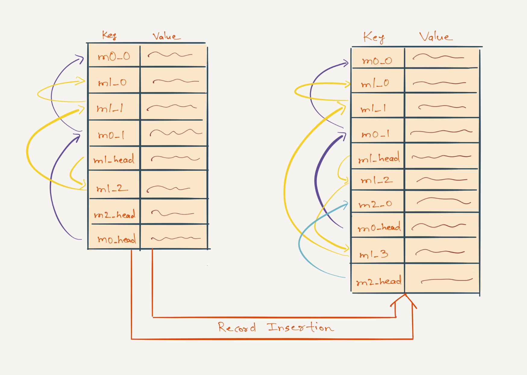
The memory used by the index node cache depends on two factors: the total number of timeline keys and the total number of records that are cached. Many timeline keys don’t have any records associated with them in the cache, because some members may not have shared new content in the feed for the past few days or may not have shared content of a certain type in the last few days. It is desirable to have good control over which timeline keys get evicted from the cache—those that have a non-empty list of records associated with them, or otherwise.
To achieve this, we use two instances of the Guava cache: one instance is called the fat cache, the other is called the skinny cache. The fat cache holds timeline keys and a non-empty list of records associated with each one of them, the skinny cache contains keys that don't have any records associated with them. The fat cache’s holding capacity is defined in terms of its ‘weight’—the total number of records it's holding, whereas the skinny cache’s holding capacity is defined in terms of its ‘size’—the total number of keys it's holding. By sizing these two instances well, we could reach the right effectiveness of caching and eviction.
Schema awareness
FollowFeed uses 
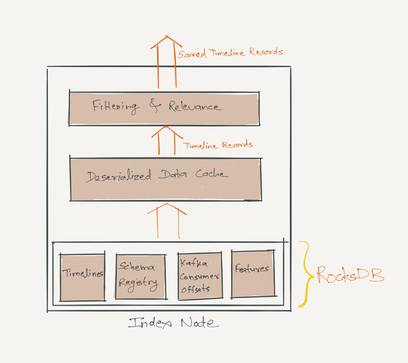
Avro as the serialization protocol for data storage. Since Avro needs reader and writer schema instances for ser/deser, we needed a schema registry that stored all versions of schemas with which the data was serialized and persisted. We chose to make the index node schema aware, which means that along with timelines, each index node also persists a Schema Registry of Avro schemas in RocksDB. This registry is used to serialize and deserialize content records. There is also an in-memory deserialized object representation of this registry to allow fast access to schema objects.
FollowFeed performs such filtering logic on records retrieved from the Guava cache. Records that pass filtering then become input to the relevance algorithms.
Relevance Computation
A key feature of FollowFeed is highly performant online relevance which ranks tens of thousands of content records per request. Low latencies are achieved by performing this relevance computation in parallel on index nodes that are serving a query. Each index node persists and caches relevance features of different entity and content types. These features are imperative in building a valid feature vector for ranking. A feature vector can be imagined as a mapping of content record onto an n-dimensional vector of numerical features.
One of the approaches we considered was to use an in-house scoring library. This library is essentially an inventory of data transformation and scoring modules, with a control flow that (1) generates a feature vector by performing a series of data transformations that parse a content record and create intermediate feature representations, and then (2) applies a regression (scoring) function to the feature vector and the model coefficient vector which is provided as input to the library. The result of the scoring function is the relevance score of the content record. Since FollowFeed scores millions of content records per second, we need the scoring function to be as efficient as possible. The data transformation steps in this library were heavy on iteration, hash-based lookups and intermediate data representation marshalling, thus these steps proved to be a bottleneck in achieving our latency SLA. At the same time, the ability to easily configure a few parameters to test and iterate through a variety of data transformations and relevance models implemented in a well-tested Java library was quite appealing. So, we came up with a new solution that retained the interface and configurability of this library, but made the implementation more efficient.
The solution was to auto-generate optimized Java code for the data transformation and scoring steps. The code generation mechanism can be thought of as being analogous to the optimization passes performed by a multi-pass compiler. However, a compiler’s optimization pass can strictly only observe the code flow without any knowledge of the inputs that may be provided to the program. Since we know the schemas of content records, and the exact data transformations and regressions that we need to perform, we can generate significantly optimized code that has certain assumptions about the input baked in. For the mobile feed use case, the optimized Java code takes about 50 microseconds (p99) to perform relevance computations on one content record, which is 15 times faster than the scoring library mentioned in the previous paragraph.
  • RocksBD
Ingestion Path
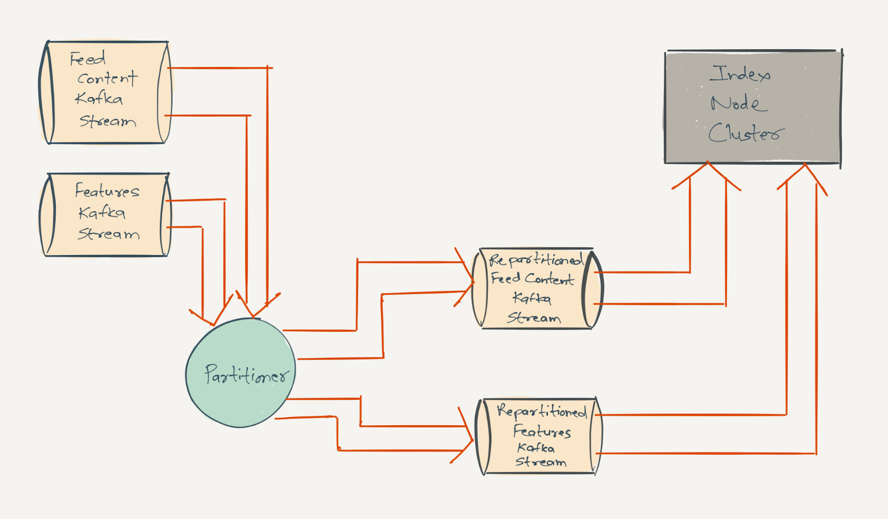
FollowFeed is designed to be eventually consistent, so all data ingestion is done asynchronously through Kafka. All the timeline data is present in a feed Kafka stream, which is a stream of all content records on LinkedIn—shares, likes, comments by members and by non-member entities such as companies, schools, etc. We have created an intermediary service called Partitioner, which consumes from the content record’s Kafka stream and republishes those events into another Kafka topic using a custom partitioning function. The resulting Kafka topic’s partition range matches the partition range of FollowFeed's index node cluster
To consume timeline data, an index node simply subscribes to the same partition range of the Kafka topic as the partition range of timeline data that it’s hosting. The use of Kafka for data ingestion into index nodes allows us to consume the data for a given partition into multiple replica index nodes thereby allowing us to easily add more replicas for a given partition set. Relevance features are similarly re-partitioned and ingested from a different Kafka stream.
As we will see below, the ease of adding more replicas results in high availability and read scalability, since all replicas serve read traffic. Also as you can probably guess at this point, the custom partitioning function used to re-partition feed events on the ingestion path is the same as the partitioning function used to route real-time queries to index nodes.
  • Partitioner
Query Path
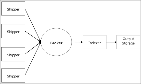
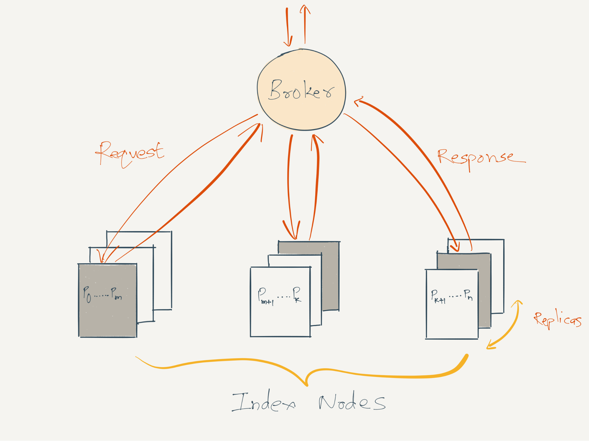
A feed query from a client is routed to the index nodes using a fan-out service called the Broker. The broker receives feed requests from a midtier service, each request includes (1) a list of entities that are of interest to the viewer, (2) use case specific filtering criteria, (3) number of content records that should be returned, and (4) viewer specific data that would be used for use case specific filtering. The broker transmutes the entities and content types it received into timeline keys and packages these timeline keys into requests for the index nodes. These requests are fanned out to the index node cluster in two steps: (1) The broker determines a mapping between the timeline keys and the partitions they belong to using the same custom partitioning function which is used on the ingestion path. (2) The broker is aware of the mapping between partitions/replicas and index nodes via D2, which is a library that provides name service and dynamic load balancing functionality using Zookeeper. Thus, the broker can now fan out requests to the appropriate index node.
The request received by an index node includes (1) a list of timeline keys whose records needs to be retrieved, (2) time range of the records that should be considered for filtering and relevance scoring, (3) number of scored timeline records that should be returned, (4) viewer specific data that would be used for filtering and (5) use case specific filtering criteria. The index node performs a batch-get and retrieves a list of content records from the underlying cache/storage using these parameters. These records undergo business logic specific filtering, and then get scored and ranked using relevance function. From the resulting ranked list of records, the requested number of records with the highest scores are returned from each index node to the broker.
Replicas in the index node cluster are set up in master-master mode. So, all replicas serve real-time read traffic.
The broker then performs a pass of business logic specific deduplication and diversity related filtering. This additional pass of filtering (besides the filtering already performed by index nodes) is required to filter out records that are too similar to each other but were returned by different index nodes. Finally, the broker sorts the filtered list of records using relevance scores, and returns the requested number of records with the highest scores to the client.
  • Broker
Multi Data Center
In the multi-data center world, different viewers can be sticky-routed to different data centers. It’s imperative that a viewer’s feed requests should be served as efficiently as possible—preferably from the data center that the viewer is sticky-routed to. This means that the timeline data of the entities that the viewer is interested in should be available in the data center locally. Since this set of entities keeps evolving continuously, we decided to replicate and store timeline data of all entities in all data centers. This is achieved by ingesting data from an aggregated Kafka stream that includes content records published from all data centers.
The size of FollowFeed’s index node clusters currently in production is primarily a function of the read traffic, so the index node cluster sizes can be different in different data centers according to the percentage of the read traffic being sticky-routed to those data centers. Each data center hosts the Partitioner service that consumes the feed updates' Kafka stream and re-partitions events. Similarly, the broker nodes routes queries to the appropriate index nodes according to the index node cluster configuration in that specific data center.
A/B Testing
A/B testing support is baked through-out the FollowFeed stack by integrating with XLNT—Linkedin’s A/B testing platform. We routinely A/B test multiple relevance models at the same time on different segments of the members, a relevance model can be chosen per viewer using a variety of criteria.
Operations: Debugging and Performance
Besides read scalability, A/B testing support, etc., a key focus during building FollowFeed was to bake operability into the system before it was launched in production.
This started with treating the persisted state mission critical and translated into the following requirements:
  • Monitoring of state: Monitoring includes real-time breakdown of the characteristics of data such as the count/rate of different content types, content types in cache versus persisted state, and also alerts on the state to catch any significant departures from the norms, etc.
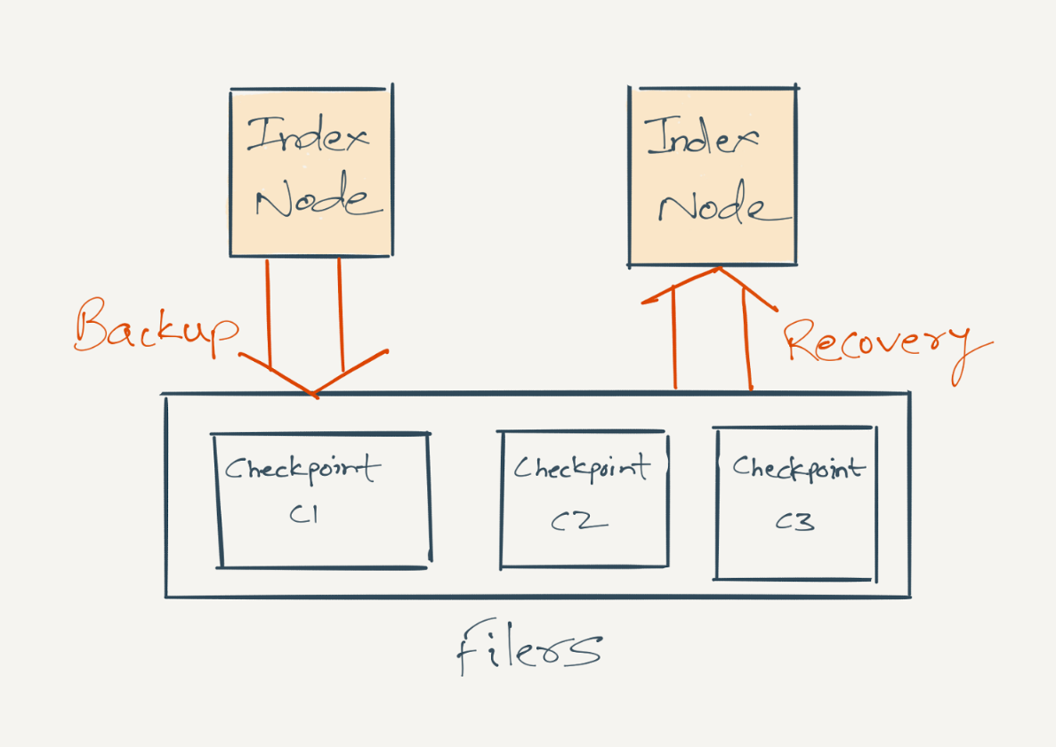
  • Recovery: Every stateful system needs the right tools to recover from state corruption. We implement this through reliable checkpointing of timeline data and recovery through backups. Data on individual storage nodes is backed up incrementally at fixed intervals to network-attached storage filers, which provide reliability through data redundancy. Backups are used to bootstrap index nodes, to bring FollowFeed clusters in new data centers online, create more replicas, etc. We also backup Kafka consumer's offsets so that during recovery, the index node can consume from Kafka from the right log offset.
  • Reliable admin tools: One-off admin tasks that affect the state should not result in outages. Tools for cluster rebalancing and re-sizing have been designed such that in case of errors the intermediate states can be safely rolled back. These tools are also continuously tested in the staging environment. We also have well-tested admin commands to retrieve and manage the state on the index nodes such as commands to (1) obtain data from the cache or the database for a specified member id, content type and time range, (2) delete cherry-picked data from the cache and/or database, (3) delete the caches entirely, (4) turn the kafka consumption on or off, etc. These tools and commands are dummy-proofed using sufficient warnings and override requirements.
  • Filer
Predictable Performance 24x7
  • To ensure that disk and network heavy operations such as backups do not interfere with real-time performance, we have a dedicated a set of index nodes that are used only for ingesting and backing up data. These nodes do not serve real-time traffic and are used for periodic backups. These nodes also host more partitions than the nodes that are serving real-time traffic.
  • The request/response loop between the broker and index nodes is asynchronous, which helps utilize broker threads more efficiently.
  • We have set an SLA on the p99 latency at the broker. If a request to the broker resulted in a request fan-out to n number of index nodes, then the broker needs to wait for responses from all of these n index nodes. In this case, higher latencies at any of these index nodes impacts the latency at the broker. To optimize this, we have put a lot of emphasis on optimizing the index node’s performance through Read-Copy-Update synchronization, concurrency control through fine-grained locking, garbage generation and collection optimization, Java cache and RocksDB configuration, TCP tunings, avoiding connection churn, page flush and swappiness optimization, etc.
  • To further mitigate the impact of higher latency percentiles at the index nodes, the broker fires duplicate requests to 1, 2, or 3 replica index nodes (all of these nodes are hosting the same set of partitions) with appropriate time-outs inserted between firing of each duplicate request. The Broker waits for responses from each of the duplicate requests and terminates the in-flight requests as soon as a response is received.
  • We leverage D2 to gracefully degrade performance in case a node gets overwhelmed with queries or its performance degrades during normal operations. D2 assigns and dynamically evaluates certain scores per broker and index node, and drops requests if the score drops below a pre-configured threshold.
  • Performance regressions are caught as early as possible: We log and plot timeouts and errors, and there are routine performance tests before deploying newer builds to production that compare timeouts and errors of the new build against the last known good build.
  • Email alerts are fired if the quality of service degrades in production due to decrease in throughput, increase in latency, exceptions, etc.
  • At times, systems see performance and timeout issues for certain requests that are not reflected in the percentile graphs. One functionality that has helped us immensely in tracking down such corner case performance (and functionality) issues is to enable TRACE level logging for certain viewers’ requests using a dynamic config. The viewer specific logging also avoids log spam and a sudden drop in performance that typically happens when log levels are changed for the entire process through a JMX “backdoor” call.
Conclusion
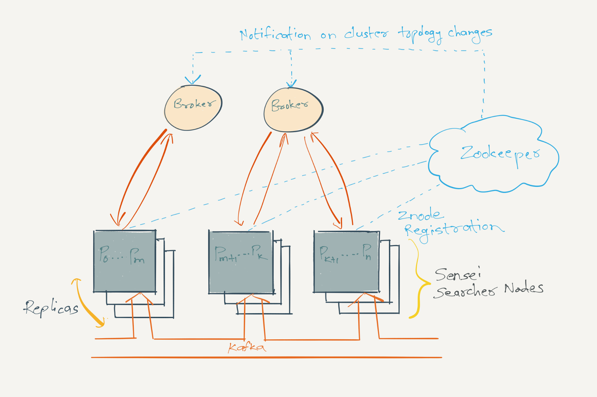
LinkedIn's newsfeed has come a long way, from just being a chronological set of records to using complex relevance algorithms to rank these records. To cater to these requirements and to support more feed queries due to an increasing user base, LinkedIn's newsfeed infrastructure has changed significantly during this time—from a generic search based solution to a more feed-optimized indexing solution. We recently finished ramping all traffic from Sensei-based architecture to FollowFeed and we have seen significant improvement in key metrics:
  • FollowFeed’s p99 latency for the mobile news feed is around 140ms which is five times faster than Sensei. As a result of this, we also saw 150ms improvement in p90 page load latency.
  • FollowFeed can host roughly 20 times more data than Sensei.
  • FollowFeed migration resulted in reducing overall capex cost by 50 percent compared to Sensei.

Labels

Review (572) System Design (334) System Design - Review (198) Java (189) Coding (75) Interview-System Design (65) Interview (63) Book Notes (59) Coding - Review (59) to-do (45) Linux (43) Knowledge (39) Interview-Java (35) Knowledge - Review (32) Database (31) Design Patterns (31) Big Data (29) Product Architecture (28) MultiThread (27) Soft Skills (27) Concurrency (26) Cracking Code Interview (26) Miscs (25) Distributed (24) OOD Design (24) Google (23) Career (22) Interview - Review (21) Java - Code (21) Operating System (21) Interview Q&A (20) System Design - Practice (20) Tips (19) Algorithm (17) Company - Facebook (17) Security (17) How to Ace Interview (16) Brain Teaser (14) Linux - Shell (14) Redis (14) Testing (14) Tools (14) Code Quality (13) Search (13) Spark (13) Spring (13) Company - LinkedIn (12) How to (12) Interview-Database (12) Interview-Operating System (12) Solr (12) Architecture Principles (11) Resource (10) Amazon (9) Cache (9) Git (9) Interview - MultiThread (9) Scalability (9) Trouble Shooting (9) Web Dev (9) Architecture Model (8) Better Programmer (8) Cassandra (8) Company - Uber (8) Java67 (8) Math (8) OO Design principles (8) SOLID (8) Design (7) Interview Corner (7) JVM (7) Java Basics (7) Kafka (7) Mac (7) Machine Learning (7) NoSQL (7) C++ (6) Chrome (6) File System (6) Highscalability (6) How to Better (6) Network (6) Restful (6) CareerCup (5) Code Review (5) Hash (5) How to Interview (5) JDK Source Code (5) JavaScript (5) Leetcode (5) Must Known (5) Python (5)

Popular Posts