assign records to nodes randomly: when you’re trying to read a particular item, you have no way of knowing which node it is on, so you would have to query all nodes in parallel.
PARTITIONING BY KEY RANGE - hot spots
assign a continuous range of keys (from some minimum to some maximum) to each partition
Within each partition, we can keep keys in sorted order.
To avoid this problem in the sensor database, you need to use something other than the timestamp as the first element of the key. For example, you could prefix each timestamp with the sensor name, so that the partitioning is first by sensor name and then by time.
PARTITIONING BY HASH OF KEY A good hash function takes skewed data and makes it uniformly distributed.
CONSISTENT HASHING
by using the hash of the key for partitioning, we also lost a nice property of key-range partitioning: the ability to do efficient range queries. Keys that were once adjacent are now scattered across all the partitions, so their sort order is lost. In MongoDB, if you have enabled hash-based sharding mode, any range query has to be sent to all partitions
Cassandra achieves a compromise between the two partitioning strategies. A table in Cassandra can be declared with a compound primary key consisting of several columns. Only the first part of that key is hashed to determine the partition, but the other columns are used as a concatenated index for sorting the data in Cassandra’s SSTables.
This means that a query cannot search for a range of values within the first column of a compound key, but if it specifies a fixed value for the first column, it can perform an efficient range scan based on the other columns of the key.
(user_id, update_timestamp)
SKEWED WORKLOADS AND RELIEVING HOT SPOTS
on a social media site, a celebrity user with millions of followers may cause a storm of activity when they do something.
it’s the responsibility of the application to reduce the skew. For example, if one key is known to be very hot, a simple technique is to add a random number to the beginning or end of the key. Just a two-digit decimal random number would split the writes to the key evenly across 100 different keys, allowing those keys to be distributed to different partitions.
However, having split the writes across different keys, any reads now have to do additional work, as they have to read the data from all 100 keys and combine it.
This technique also requires additional bookkeeping: it only makes sense to append the random number for the small number of hot keys; for the vast majority of keys with low write throughput this would be unnecessary overhead. Thus, you also need some way of keeping track which keys are being split.
Partitioning and secondary indexes
The problem with secondary indexes is that they don’t map neatly to partitions. PARTITIONING SECONDARY INDEXES BY DOCUMENT each partitions maintains its own secondary indexes, covering only the documents in that partition. It doesn’t care what data is stored in other partitions. a document-partitioned index is also known as a local index. This approach to querying a partitioned database is sometimes known as scatter/gather, and it can make read queries on secondary indexes quite expensive. Even if you query the partitions in parallel, scatter/gather is prone to tail latency amplification.
MongoDB, Riak, Cassandra, Elasticsearch, SolrCloud, and VoltDB all use document-partitioned secondary indexes.
PARTITIONING SECONDARY INDEXES BY TERM A global index must also be partitioned, but it can be partitioned differently from the primary key index. The advantage of a global (term-partitioned) index over a document-partitioned index is that it can make reads more efficient: rather than doing scatter/gather over all partitions, a client only needs to make a request to the partition containing the term that it wants. However, the downside of a global index is that writes are now slower and more complicated, because a write to a single document may now affect multiple partitions of the index (every term in the document might be on a different partition, on a different node).
In practice, updates to global secondary indexes are often asynchronous (that is, if you read the index shortly after a write, the change you just made may not yet be reflected in the index).
For example, Amazon DynamoDB states that its global secondary indexes are updated within a fraction of a second in normal circumstances, but may experience longer propagation delays in case of faults in the infrastructure.
Rebalancing partitions
How not to do it: hash mod N Fixed number of partitions - good for hash partitioning create many more partitions than there are nodes, and assign several partitions to each node.
Only entire partitions are moved between nodes. The number of partitions does not change, nor does the assignment of keys to partitions change. The only thing that changes is the assignment of partitions to nodes.
This change of assignment is not immediate—it takes some time to transfer a large amount of data over the network—so the old assignment of partitions is used for any reads and writes that happen while the transfer is in progress.
by assigning more partitions to nodes that are more powerful, you can force those nodes to take a greater share of the load.
This approach to rebalancing is used in Riak, Cassandra since version 1.2, Elasticsearch, Couchbase and Voldemort.
Dynamic partitioning - both key-range-partitioned databases such as HBase and RethinkDB create partitions dynamically. When a partition grows to exceed a configured size, it is split into two partitions so that approximately half of the data ends up on each side of the split. Conversely, if lots of data is deleted and a partition shrinks below some threshold, it can be merged with an adjacent partition. the number of partitions adapts to the total data volume.
HBase and MongoDB allow an initial set of partitions to be configured on an empty database (this is called pre-splitting).
Before version 1.2, Cassandra used consistent hashing with pseudo-random partition boundaries, as originally described by Karger et al. Rather than assigning several small partitions to each node, it used one big partition per node, covering a large continuous range of hashes.
However, this approach suffered from poor load distribution, and made it difficult to add nodes to the cluster: an existing node had to split its range to give half of its data to a new node. This expensive operation was difficult to perform in the background without impacting query performance. For those reasons, Cassandra’s partitioning strategy was replaced with the fixed-number-of-partitions approach described above.
the most widely-used partitioning models are either hashing with a fixed number of partitions, or dynamic partitioning by key range (when range queries are required).
OPERATIONS: AUTOMATIC OR MANUAL REBALANCING AUTOMATIC REBALANCING can be dangerous in combination with automatic failure detection.
Request routing Allow clients to contact any node (e.g. via a round-robin load balancer). If that node coincidentally owns the partition to which the request applies, it can handle the request directly; otherwise it forwards the request to the appropriate node. Send all requests from clients to a routing tier first, which determines the node that should handle the request and forwards it accordingly. This routing tier does not itself handle any requests, it only acts as a partition-aware load balancer. Require that clients be aware of the partitioning and the assignment of partitions to nodes. In this case, a client can connect directly to the appropriate node, without any intermediary.
Many distributed data systems rely on a separate coordination service such as Zookeeper to keep track of this cluster metadata. Each node registers itself in Zookeeper, and Zookeeper maintains the authoritative mapping of partitions to nodes.
Other actors, such as the routing tier or the partitioning-aware client, can subscribe to this information in Zookeeper. Whenever a partition changes ownership, or a node is added or removed, Zookeeper notifies the routing tier so that it can keep its routing information up-to-date.
LinkedIn’s Espresso uses Helix for cluster management (which in turn relies on Zookeeper), implementing a routing tier. HBase, SolrCloud and Kafka also use Zookeeper to track partition assignment.
Cassandra and Riak take a different approach: they use a gossip protocol among the nodes to disseminate and agree on any changes in cluster state. Requests can be sent to any node, and that node forwards them to the appropriate node for the requested partition. This puts more complexity in the database nodes, but avoids the dependency on an external coordination service such as Zookeeper.
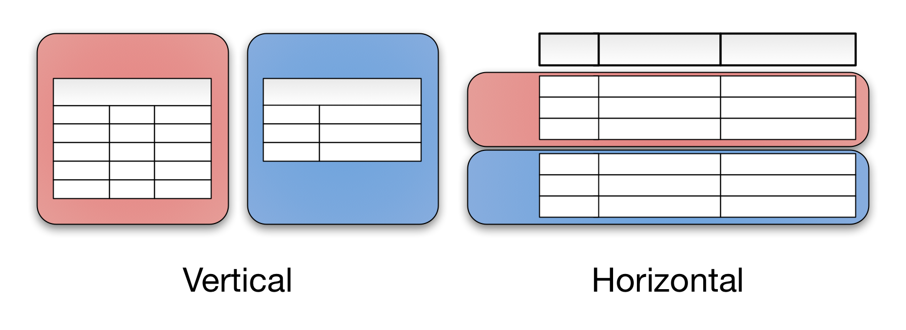
PARALLEL QUERY EXECUTION https://medium.com/@jeeyoungk/how-sharding-works-b4dec46b3f6 Sharding is also referred ashorizontal partitioning. The distinction of horizontal vsverticalcomes from the traditional tabular view of a database. A database can be split vertically — storing different tables & columns in a separate database, or horizontally — storing rows of a same table in multiple database nodes.
Vertical partitioning is very domain specific. You draw a logical split within your application data, storing them in different databases. It is almost always implemented at the application level — a piece of code routing reads and writes to a designated database.
Case 1 — Algorithmic Sharding
One way to categorize sharding is algorithmic versus dynamic. In algorithmic sharding, the client can determine a given partition’s database without any help. In dynamic sharding, a separate locator service tracks the partitions amongst the nodes.
An algorithmically sharded database, with a simple sharding function
Algorithmically sharded databases use a sharding function (partition_key) -> database_id to locate data. A simple sharding function may be “hash(key) % NUM_DB”.
Reads are performed within a single database as long as a partition key is given. Queries without a partition key require searching every database node. Non-partitioned queries do not scale with respect to the size of cluster, thus they are discouraged.
Algorithmic sharding distributes data by its sharding function only. It doesn’t consider the payload size or space utilization. To uniformly distribute data, each partition should be similarly sized. Fine grained partitions reduce hotspots — a single database will contain many partitions, and the sum of data between databases is statistically likely to be similar. For this reason, algorithmic sharding is suitable for key-value databases with homogeneous values.
Resharding data can be challenging. It requires updating the sharding function and moving data around the cluster. Doing both at the same time while maintaining consistency and availability is hard. Clever choice of sharding function can reduce the amount of transferred data. Consistent Hashing is such an algorithm.
Examples of such system include Memcached. Memcached is not sharded on its own, but expects client libraries to distribute data within a cluster. Such logic is fairly easy to implement at the application level.
Case 2— Dynamic ShardingIn dynamic sharding, an external locator service determines the location of entries. HDFS uses a Name Node to store filesystem metadata. Unfortunately, the name node is a single point of failure in HDFS. Apache HBase splits row keys into ranges. The range server is responsible for storing multiple regions. Region information is stored in Zookeeper to ensure consistency and redundancy. In MongoDB, the ConfigServer stores the sharding information, and mongos performs the query routing. ConfigServer uses synchronous replication to ensure consistency. When a config server loses redundancy, it goes into read-only mode for safety. Normal database operations are unaffected, but shards cannot be created or moved.Case 3 — Entity Groups
The concept of entity groups is very simple. Store related entities in the same partition to provide additional capabilities within a single partition. Specifically:
Queries within a single physical shard are efficient.
Stronger consistency semantics can be achieved within a shard.
Case 4 — Hierarchical keys & Column-Oriented DatabasesColumn-oriented databases are an extension of key-value stores. They add expressiveness of entity groups with a hierarchical primary key. A primary key is composed of a pair (row key, column key). Entries with the same partition key are stored together. Range queries on columns limited to a single partition are efficient. That’s why a column key is referred as a range key in DynamoDB.http://ayende.com/blog/134145/sharding-vs-having-multiple-databases https://www.quora.com/Whats-the-difference-between-sharding-and-partition
Partitioning is a general term used to describe the act of breaking up your logical data elements into multiple entities for the purpose of performance, availability, or maintainability.
Sharding is the equivalent of "horizontal partitioning". When you shard a database, you create replica's of the schema, and then divide what data is stored in each shard based on a shard key. For example, I might shard my customer database using CustomerId as a shard key - I'd store ranges 0-10000 in one shard and 10001-20000 in a different shard. When choosing a shard key, the DBA will typically look at data-access patterns and space issues to ensure that they are distributing load and space across shards evenly.
"Vertical partitioning" is the act of splitting up the data stored in one entity into multiple entities - again for space and performance reasons. For example, a customer might only have one billing address, yet I might choose to put the billing address information into a separate table with a CustomerId reference so that I have the flexibility to move that information into a separate database, or different security context, etc.
To summarize - partitioning is a generic term that just means dividing your logical entities into different physical entities for performance, availability, or some other purpose. "Horizontal partitioning", or sharding, is replicating the schema, and then dividing the data based on a shard key. "Vertical partitioning" involves dividing up the schema (and the data goes along for the ride).
Final note: you can combine both horizontal and vertical partitioning techniques - sometimes required in big data, high traffic environments.
Multi-master replication can be contrasted with master-slave replication, in which a single member of the group is designated as the "master" for a given piece of data and is the only node allowed to modify that data item. Other members wishing to modify the data item must first contact the master node. Allowing only a single master makes it easier to achieve consistency among the members of the group, but is less flexible than multi-master replication.
Multi-master replication can also be contrasted with failover clustering where passive slave servers are replicating the master data in order to prepare for takeover in the event that the master stops functioning. The master is the only server active for client interaction.
The primary purposes of multi-master replication are increased availability and faster server response time.
If one master fails, other masters continue to update the database.
Masters can be located in several physical sites, i.e. distributed across the network.
Most multi-master replication systems are only loosely consistent, i.e. lazy and asynchronous, violating ACID properties.
Eager replication systems are complex and increase communication latency.
Issues such as conflict resolution can become intractable as the number of nodes involved rises and latency increases.
databaseclusters implement multi-master replication using one of two methods. Asynchronous multi-master replication commits data changes to a deferred transaction queue which is periodically processed on all databases in the cluster. Synchronous multi-master replication uses Oracle's two phase commit functionality to ensure that all databases with the cluster have a consistent dataset.
 Vertical partitioning is very domain specific. You draw a logical split within your application data, storing them in different databases. It is almost always implemented at the application level — a piece of code routing reads and writes to a designated database.