a QUORUM read requires consulting with at least two out of three replicas, it is easy to see how this query will result in consulting many nodes. In the following diagram, our client makes a request to one of the nodes, which will act as coordinator. The coordinator must then make requests to at least two replicas for each key in the query:
The end result is that we require four out of six nodes to fulfill this query! If any one of these calls fails, the entire query will fail. It is easy to see how a query with many keys could require participation from every node in the cluster.
When using the IN clause, it's best to keep the number of keys small. There are valid use cases for this clause, such as querying across time buckets for time series models, but in such cases, you should try to size your buckets such that you only need at most two in order to fulfill the request.
it is often advisable to issue multiple queries in parallel as opposed to utilizing the IN clause. While the IN clause may save you from multiple network requests to Cassandra, the coordinator must do more work. You can often reduce overall latency and workload with several token-aware queries as you'll be talking directly to the nodes that contain the data.
When using the IN clause, if any one key times out, you will have to retry the entire query.
SELECT * FROM authors WHERE publisher = 'Putnam'; InvalidRequest: code=2200 [Invalid query] message="Cannot execute this query as it might involve data filtering and thus may have unpredictable performance. If you want to execute this query despite the performance unpredictability, use ALLOW FILTERING"
Because we have not specified the partition key, this query will require a full, distributed table scan
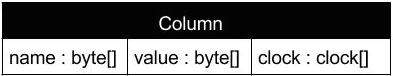
At the storage layer, a secondary index is simply another table, where the key is the value of the indexed column, and the columns contain the row keys of the indexed table
So a query filtering on publisher will use the index to each author name, and then query all the authors by key. This is similar to using the IN clause, since we must query replicas for every key with an entry in the index.
Cassandra co-locates index entries with their associated original table keys.
Cassandra - local index
The objective of using this approach is to be able to determine which nodes own indexed keys, as well as to obtain the keys themselves in a single request. But the problem is that we have no idea which token ranges contain indexed keys until we ask each range.
the use of secondary indices has an enormous impact on both performance and availability, since all nodes must participate in fulfilling the query. While this could be acceptable for occasional queries, trying to do it with critical, high-volume queries will be problematic. In a distributed system with many nodes, there is a high likelihood that at least one node will be unable to respond. For this reason, it's best to avoid using them in favor of materialized views or another data model entirely.
make sure you only index on low-cardinality values, as high-cardinality indices do not scale well. But don't go so low that your index is rendered useless. For example, booleans are bad, as are UUIDs, but birth year could be a reasonable column to index.
Modeling for Availability SSTable Attached Secondary Index (SASI) The index is attached to the SSTable itself, rather than being relegated to a separate table. This means the read path is much more straightforward, requiring only a single pass to read both the index and the underlying data.
CREATE CUSTOM INDEX authors_publisher
ON authors(publisher) USING 'org.apache.cassandra.index.sasi.SASIIndex';
Distributed joins
If you find yourself querying multiple large tables and then joining them in your application based on some shared key, you are performing a distributed join. This should almost always be avoided in favor of a denormalized data model. The only exception is for very small lookup tables that can fit easily in memory. Otherwise, you should always write your data the way you intend to read it.
Resurrecting the dead
Let's assume that multiple replicas exist for a given column, yet only one has recorded the tombstone. If one of the nodes remains down past gc_grace_seconds without a repair operation, when it finally comes back online, it will still contain the old data and be unaware of the delete. Any subsequent repair will then recreate the old data on other nodes as if the delete had never occurred.
To ensure that deleted data never resurfaces, make sure you run repair at least once every gc_grace_seconds, and never let a node stay down for longer than this time period.
The last write win
old values must periodically be purged to avoid accumulating unnecessary junk data over time
Compaction aggregates partitions from multiple files into a single file, and in the process it removes old data and purges tombstones. the other objective is to improve read performance by moving data for a given key into a single SSTable, thereby reducing the disk I/O required to read each key.
Size-tiered compaction: This strategy causes SSTables to be compacted when there are multiple files of a similar size (the default is four). In update-heavy workloads, a partition may exist in many SSTables at once, resulting in reduced read performance.
SSTables are chosen for compaction based on size buckets.
It can require a lot of extra disk space, as much as twice the used disk space if there are no deletes or updates. This is because the tables are copied during compaction, so the data will be duplicated while the process is running. This is especially important for operations because it means you must have as much free space as your largest SSTables or they won't be able to compact.
A row can exist in multiple SSTables, which can result in degradation of read performance. This is especially true if you perform many updates or deletes.
If you have very write-heavy workloads or your writes are generally immutable, size-tiered compaction can be a good strategy. Otherwise, you should probably choose leveled or time-window compaction.
When the compaction process finds multiple SSTables (the default is four) of a similar size, it will compact those tables into a single SSTable. Eventually, there will be four larger tables, which will be compacted again into one table.
Size tiered compaction strategy combine multiple SSTables which belong to a particular data size range.
This technique categories SSTables into different buckets and compaction process will run for each bucket indiviaully.
Sort SSTable according to size in descending order. After sorting above SStable we will have a list of sorted SSTables(in MB) as 100, 78, 60, 51, 34, 27, 19, 10, 7, 1.
Categories SSTables into a multiple buckets based on configuration and following condition : IF ((bucket avg size * bucket_low < SStable’ size < bucket avg size * bucket_high) OR (SStable’ size < min_sstable_size AND bucket avg size < min_sstable_size)) then add the SSTable to the bucket and compute the new avg. size of the bucket. ELSE create a new bucket with the SSTable.
Buckets are sorted according to their hotness(CASSANDRA-5515) property. Hotness of bucket is sum of hotness of SSTables in bucket. Cold bucket will get the less priority than hot buckets for compaction.
Those buckets do not meet the criteria of min_threshold will be discarded. Those buckets have SSTables more than max_threshold, will be trimmed to max_threshold and appear for the compaction. All SSTables in such bucket will be sorted according to hotness of SSTable and top (32/ max_threshold ) SStable will be considered.
Limitation:
Size tiered compaction doesnt give any guarantee about column distribution of particular row. I may possible that columns of particular row-key belong to different SSTables. In such cases read performance will hit as read operation need to touch all SSTables where columns present.
In worst case it might need exact amount of free space(100%) to combine SSTables.
Keeping a count of reads per-sstable would allow STCS to automatically ignore cold data rather than recompacting it constantly with hot data, dramatically reducing compaction load for typical time series applications and others with time-correlated access patterns. We would not need a separate age-tiered compaction strategy.
Leveled compaction: This strategy assigns SSTables to levels, where each level represents tables that are 10 times larger than the next lower level. This guarantees that tables in the same level won't overlap, and results in the vast majority of rows being read from a single SSTable. This is good for read-heavy workloads, but if you don't perform updates or deletes, or query large ranges across a partition, the additional I/O may not be worth the cost.
leveled compaction attempts to create SSTables that are fixed in size and then grouped into levels based on their size, with each level being 10 times the size of the previous level. A key trait of leveled compaction is that within a level, there are no overlapping SSTables. This minimizes the number of files that need to be checked in a given level, because a partition can only exist in at most one (and most likely zero) SSTable per level.
The algorithm is straightforward. New SSTables are placed in the first level, called L0, after which they are immediately compacted with the overlapping tables in the next level, L1. As L1 becomes filled, extra tables are merged with tables in L2, and so on.
This process introduces several improvements over size-tiered compaction for workloads involving lots of reads or updates:
It uses much less space than size-tiered compaction, reducing the amount of disk space used while the SSTable is being compacted. Since SSTables are also much smaller using this strategy, this amounts to a reduction in space complexity.
Much less space is wasted by old rows, at most 10%.
Read performance is often improved, as 90% of all reads will require a lookup in only a single SSTable.
The leveled compaction strategy actually employs a hybrid approach, where the process switches to size-tiered compaction when Cassandra is unable to keep up with the load. The max_threshold property determines when this occurs.
Thus, over time, many versions of a row may exist in different sstables. Each of these versions may have different sets of columns. If the sstables were allowed to accumulate, reading a row could require many seeks in different files to return a result.
To prevent read speed from deteriorating, compaction runs in the background, merging sstables together. (This can also be done performantly, without random i/o, because rows are sorted by primary key within in each sstable.)
There are three problems with size-tiered compaction in update-heavy workloads:
Performance can be inconsistent because there are no guarantees as to how many sstables a row may be spread across: in the worst case, we could have columns from a given row in each sstable.
A substantial amount of space can be wasted since there is no guarantee as to how quickly obsolete columns will be merged out of existance; this is particularly noticeable when there is a high ratio of deletes.
Space can also be a problem as sstables grow larger from repeated compactions, since an obsolete sstable cannot be removed until the merged sstable is completely written. In the worst case of a single set of large sstable with no obsolete rows to remove, Cassandra would need 100% as much free space as is used by the sstables being compacted, into which to write the merged one.
Leveled compaction creates sstables of a fixed, relatively small size (5MB by default in Cassandra's implementation), that are grouped into "levels." Within each level, sstables are guaranteed to be non-overlapping. Each level is ten times as large as the previous.
In figure 3, new sstables are added to the first level, L0, and immediately compacted with the sstables in L1 (blue). When L1 fills up, extra sstables are promoted to L2 (violet). Subsequent sstables generated in L1 will be compacted with the sstables in L2 with which they overlap. As more data is added, leveled compaction results in a situation like the one shown in figure 4.
Figure 4: sstables under leveled compaction after many inserts
This solves the above problems with tiered compaction:
Leveled compaction guarantees that 90% of all reads will be satisfied from a single sstable (assuming nearly-uniform row size). Worst case is bounded at the total number of levels -- e.g., 7 for 10TB of data.
At most 10% of space will be wasted by obsolete rows.
Only enough space for 10x the sstable size needs to be reserved for temporary use by compaction.
Because leveled compaction makes the above guarantees, it does roughly twice as much i/o as size-tiered compaction. For primarily insert-oriented workloads, this extra i/o does not pay off in terms of the above benefits, since there are few obsolete row versions involved.
Leveled compaction ignores the concurrent_compactors setting. Concurrent compaction is designed to avoid tiered compaction's problem of a backlog of small compaction sets becoming blocked temporarily while the compaction system is busy with a large set. Leveled compaction does not have this problem, since all compaction sets are roughly the same size. Leveled compaction does honor the multithreaded_compaction setting, which allows using one thread per sstable to speed up compaction. However, most compaction tuning will still involve using compaction_throughput_mb_per_sec (default: 16) to throttle compaction back.
In addition to lowering read latencies in general, leveled compaction lowers the amount of variability in read latencies. If your application has strict latency requirements for the 99th percentile, leveled compaction may be the only reliable way to meet those requirements, because it gives you a known upper bound on the number of SSTables that must be read.
High Read/Write Ratio
If you perform at least twice as many reads as you do writes, leveled compaction may actually save you disk I/O, despite consuming more I/O for compaction. This is especially true if your reads are fairly random and don't focus on a single, hot dataset.
Rows Are Frequently Updated
Whether you're dealing with skinny rows where columns are overwritten frequently (like a "last access" timestamp in a Users column family) or wide rows where new columns are constantly added, when you update a row with size-tired compaction, it will be spread across multiple SSTables. Leveled compaction, on the other hand, keeps the number of SSTables that the row is spread across very low, even with frequent row updates.
If you're using wide rows, switching to a new row periodically can alleviate some of the pain of size-tiered compaction, but not to the extent that leveled compaction can. If you're using short rows, Cassandra 1.1 does have a new optimization for size-tiered compaction that helps to merge fragmented rows more quickly (though it does not reclaim the disk space used by those fragments).
Deletions or TTLed Columns in Wide Rows
When Leveled Compaction may not be a Good Option
Your Disks Can't Handle the Compaction I/O
If your cluster is already pressed for I/O, switching to leveled compaction will almost certainly only worsen the problem. This is the primary downside to leveled compaction and the main problem you should check for in advance; see the notes below about write sampling.
Write-heavy Workloads
It may be difficult for leveled compaction to keep up with write-heavy workloads, and because reads are infrequent, there is little benefit to the extra compaction I/O.
LeveledCompactionStrategy (LCS) in Cassandra implements the internals of LevelDB. You can check the exact implementation details in LevelDB implementation doc.
In order to give you a simple explanation take into account the following points:
Every sstable is created when a fixed (relatively small) size limit is reached. By default L0 gets 5MB files of files, and each subsequent level is 10x the size. (in L1 you'll have 50MB of data, L2 500MB, and so on).
Sstables are created with the guarantee that they don't overlap
When a level fills up, a compaction is triggered and stables from level-L are promoted to level-L+1. So, in L1 you'll have 50MB in ~10 files, L2 500MB in ~100 files, etc..
In bold are the relevant details that justify the 90% reads from the same file (sstable). Let's do the math together and everything will become clearer (I hope :)
Imagine you have keys A,B,C,D,E in L0, and each keys takes 1MB of data.
Next we insert key F. Because level 0 is filled a compaction will create a file with [A,B,C,D,E] in level 1, and F will remain in level 0.
That's ~83% of data in 1 file in L1
Next we insert G,H,I,J and K. So L0 fills up again, L1 gets a new sstable with [I,G,H,I,J].
By now we have K in L0, [A,B,C,D,E] and [I,G,H,I,J] in L1
And that's ~90% of data in L1 :)
If we continue inserting keys we will get around the same behavior so, that's why you get 90% of reads served from roughly the same file/sstable.
Time-window compaction - time series, with TTLs
this strategy replaces the deprecated date-tiered compaction, which suffered from usability and performance issues. It groups SSTables by time bucket and expiration, thereby allowing the compaction process to simply drop expired tables and ignore old unexpired tables. This strategy can dramatically reduce cluster overhead for time series workloads.
groups data into SSTables based on the write time and expiration. This can be helpful for time series models where the most frequent query patterns involve reading the most recent data. If you use TTLs, this strategy can group data expiring at the same time into the same SSTables, which allows it to simply remove the table without having to run compaction. Time-window compaction makes use of size-tiered compaction within windows, so it supports all the existing size-tiered configuration options.
Date-tiered compaction:Deprecated as of 3.8 in favor of the more straightforward time-window strategy.
you can choose to throttle it using the compaction_throughput_mb_per_sec setting in cassandra.yaml. The default is 16 MB/sec, which may be sufficient for many workloads
CQL data representation does not always match the underlying storage structure.
- Each column also has a timestamp that is used for conflict resolution.
row key is distributed randomly using a hash algorithm, so the results are returned in no particular order
columns are stored in sorted order by name, using the natural ordering of the type
primary key partition keys vs clustering columns
When declaring a primary key, the first field in the list is always the partition key. This translates directly to the storage row key, which is randomly distributed in the cluster via the hash algorithm. Most queries require that you provide the partition key, so that Cassandra will know which nodes contain the requested data.
The remaining fields in the primary key declaration are called clustering columns, and these determine the ordering of the data on disk. But they play a key role in determining the kinds of queries you can run against your data
the new storage engine (as of 3.0) provides optimizations to avoid duplication of the clustering column names.
CREATE TABLE authors (
name text,
year int,
title text,
isbn text,
publisher text,
PRIMARY KEY (name, year, title)
);
name | year | title | isbn | publisher
------------+------+-----------------+---------------+-----------
Tom Clancy | 1987 | Patriot Games | 0-399-13241-4 | Putnam
Tom Clancy | 1993 | Without Remorse | 0-399-13825-0 | Putnam
our two CQL rows translated to a single storage row, because both of our inserts used the same partition key
The location of our year and title column values. They are stored as parts of the column name, rather than column values! Note that this is a simplified representation, as the new storage engine (as of 3.0) provides optimizations to avoid duplication of the clustering column names.
WITH CLUSTERING ORDER BY (year DESC);
COMPOSITE PARTITION KEYS
The most common reason for doing this is to improve data distribution characteristics. A prime example of this is the use of time buckets as keys when modeling time series data.
PRIMARY KEY ((name, year), title)
move the year from a component of the column name to a component of the row key
Row Key: Tom Clancy:1993
=> (name=Without Remorse:isbn, value=0-399-13241-4)
=> (name=Without Remorse:publisher, value=5075746e616d)
-------------------
Row Key: Tom Clancy:1987
=> (name=Patriot Games:isbn, value=0-399-13825-0)
=> (name=Patriot Games:publisher, value=5075746e616d)
The 3.0 release introduced a significant refactor of the storage engine. Previously, the storage engine had no concept of CQL rows but rather represented data as a simple map of binary keys to binary cell blobs. The new engine understands the CQL rows, clustering columns, and type information, which allows for a number of improvements in both space and computational efficiency.
Cassandra doesn't allow ad hoc queries of the sort that you can perform using SQL on a relational system
You must choose your partition key carefully, because it must be known at query time and must also distribute well across the cluster. Make sure to avoid models where even a small number of keys will contain huge numbers of columns, as this will impact data distribution.
it is not possible to perform range queries across multiple partitions as they are located in physically different places on disk.
You have to carefully order your clustering columns, because the order affects the sort order of your data on disk and therefore determines the kinds of queries you can perform.
structure your data in terms of your queries
Denormalizing using collections - sets, lists, and maps
The size of each item in a collection must not be more than 64 KB
A maximum of 64,000 items may be stored in a single collection
Querying a collection always returns the entire collection
Collections are best used for relatively small, bounded datasets
Set
- stores them in their natural sort order
- At the storage layer, set values are stored as column names, with the values left blank
books set<text>
INSERT INTO authors (name, books) VALUES ('Tom Clancy', {'Without Remorse', 'Patriot Games'});
UPDATE authors SET books = books + {'Red Storm Rising'} WHERE name = 'Tom Clancy';
UPDATE authors SET books = books - {'Red Storm Rising'} WHERE name = 'Tom Clancy';
books list<text>
INSERT INTO authors (name, books) VALUES ('Tom Clancy', ['Without Remorse', 'Patriot Games']);
Unlike set, the list structure at the storage layer places the list item in the column value, and the column name instead contains a UUID for ordering purposes.
books map<text, int>,
INSERT INTO authors (name, books) VALUES ('Tom Clancy', {'Without Remorse':1993, 'Patriot Games':1987});
UPDATE authors SET books['Red Storm Rising'] = 1986 WHERE name = 'Tom Clancy';
DELETE books['Red Storm Rising'] FROM authors WHERE name = 'Tom Clancy';
RowKey: Tom Clancy
=> (name=books:50617472696f742047616d6573, value=000007c3)
=> (name=books:576974686f75742052656d6f727365, value=000007c9)
Denormalizing with materialized views read data using an alternate key entirely. In order to be able to read your data by partition key, and in sorted order, it is often necessary to write data in more than one way
CREATE MATERIALIZED VIEW books_by_year AS SELECT * FROM authors WHERE year IS NOT NULL AND name IS NOT NULL AND title IS NOT NULL PRIMARY KEY (year, name, title);
CQL requires us to specify a non-null query predicate for each of the primary key columns. In the previous example we simply used the IS NOT NULL qualifier, but it is also possible to filter data using the WHERE clause
whenever data is modified, as Cassandra must now perform writes to both the base table and the view table(s)
updates to views are atomic, so there is no concern about data getting out of sync.
Designing for immutability
relational data tends to be mutable whereas time series data is generally immutable
- add a time component to your data model
examine our intended query patterns first
CREATE TABLE sensor_readings (
sensorID uuid,
timestamp bigint,
reading decimal,
PRIMARY KEY (sensorID, timestamp)
) WITH CLUSTERING ORDER BY (timestamp DESC);
- problematic,
If we presume that sensors will continue to collect data indefinitely, the result of this data model will be unbounded row growth. This is because each new CQL row for a given sensor is actually adding columns to the same storage row. Eventually this model will result in an unsustainable number of columns in each row, with no easy way to archive off old data.
Using a sentinel value
CREATE TABLE sensor_readings (
sensorID uuid,
time_bucket int,
timestamp bigint,
reading decimal,
PRIMARY KEY ((sensorID, time_bucket), timestamp)
) WITH CLUSTERING ORDER BY (timestamp DESC);
When choosing values for your time buckets, a rule of thumb is to select an interval that allows you to perform the bulk of your queries using only two buckets. The more buckets you query, the more nodes will be involved to produce your result.
SELECT * FROM sensor_readings
WHERE sensorID = 53755080-4676-11e4-916c-0800200c9a66
AND time_bucket = 1411840800 LIMIT 1;
SELECT * FROM sensor_readings
WHERE sensorID = 53755080-4676-11e4-916c-0800200c9a66
AND time_bucket IN (1411840800, 1411844400)
AND timestamp >= 1411841700
AND timestamp <= 1411845300;
avoid hotspot
simply get a list of the latest readings from all sensors.
It would be tempting to simply remove sensorID from the primary key, using only time_bucket as the partition key. The problem with this strategy is that all writes and most reads would be against a single partition key.
you determine some sentinel value that can be used in place of the sensorID, and that is not time oriented. For example, sensor type or a hash of the sensorID could be a good value.
In practice I have found that this use case is rare, or that the real use case requires a queue or cache. Using Cassandra, or most databases for that matter, as a queue is an antipattern
geospatial data - find points near a given location
- geohashing
- A geohash is a base-32 representation of a geographic area, where each additional digit represents greater precision. The property of geohashes that makes them particularly suited for geospatial searches is that adding a level of precision to a given geohash results in an area contained within the lower-precision value.
To find a key that can be used to narrow down the potential list of locations, and to avoid querying many keys at once.
we can use a low-precision geohash as the partition key, and then the full geohash can be stored as a clustering column. The chosen precision will determine how many keys must be queried to produce results to fill the search space
CREATE TABLE geo_search (
geo_key text,
geohash text,
place_name text, PRIMARY KEY (geo_key, geohash)
);
INSERT INTO geo_search (geo_key, geohash, place_name) VALUES ('dnh03', 'dnh03pt4', 'Green Grocery Store');
If necessary, you can also insert values with keys at multiple precision levels, enabling either coarse- or fine-grained queries. To query for points near a location, you can simply compute the geohash of the location, then truncate it to the precision level of the key. Once you have this value, a simple select produces the desired results.
SELECT * FROM geo_search WHERE geo_key = 'dnh03';
You can also easily imagine combining geohashing with time series data to keep track of location changes over time. This can be accomplished by creating a partition key consisting of time bucket and low-precision geohash. This model allows for querying a range of time for a given location.
All requests were executed synchronously, as Thrift has no built-in support for asynchronous calls.
CQL
- cursors, batches, prepared statements, and cluster awareness
- the Thrift server is now disabled by default, and re-enabling it requires modifying cassandra.yaml or using nodetool enablethrift.
cassandra-driver-core
cluster = Cluster.builder()
.addContactPoints("10.10.10.1", "10.10.10.2", "10.10.10.3")
.build();
You should only have one instance of Cluster in your application for each physical cluster, as this class controls the list of contact points and key connection policies such as compression, failover, request routing, and retries.
Use prepared statements whenever you need to execute the same statement repeatedly, as this will reduce parsing overhead on the server. However, do not create the same prepared statement multiple times, as this will actually degrade performance. You should prepare statements only once and reuse them for multiple executions.
BatchStatement
They are atomic, but not isolated: This means clients will be able to see the incremental updates as they happen. The exception is updates to a single partition, which are isolated.
They are slower
- To avoid this penalty you can use unlogged batches, which turn off atomicity and provide increased performance over multiple statements executed against the same partition.
They are unordered: Batching applies the same timestamp to all mutations in the batch, so statements don't actually execute in the provided ordering.
Be careful when using them with prepared statements to update many sparse columns: It's tempting to prepare a single statement with a number of parameters for use in a large batch. This works fine if you always supply all the parameters, but don't assume you can insert nulls for missing columns, as inserting nulls creates tombstones.
ResultSetFuture f = session.executeAsync(query);
ResultSet rs = f.getUninterruptibly();
Future<List<ResultSet>>future = Futures.allAsList(
session.executeAsync(q1),
session.executeAsync(q2)
List<ResultSet> results = future.get(5, TimeUnit.SECONDS);
A call to ResultSetFuture.getUninterruptibly() will throw helpful Cassandra-specific exceptions, while Future.get() throws the more generic ExecutionException and TimeoutException. It's also worth noting that the Future returned by allAsList() will only be successful if all component Future succeed.
the native driver connects to the cluster and learns about the topology of the ring.
Cluster.getMetadata()
RoundRobinPolicy, DCAwareRoundRobinPolicy
DCAwareRoundRobinPolicy: This policy also executes in a round-robin fashion, but ensures that requests are routed only to hosts in the local data center. Keep in mind that this does NOT obviate the need to satisfy cross-data center consistency levels (such as QUORUM). It merely limits client connections to local nodes. This policy is the default lower-level policy and is typically wrapped by a higher-level implementation.
LatencyAwarePolicy
WhiteListPolicy
TokenAwarePolicy
The default combination of the DCAwareRoundRobinPolicy wrapped by the TokenAwarePolicy
Failing over to a remote data center
Downgrading consistency level
.withRetryPolicy(DowngradingConsistencyRetryPolicy.INSTANCE)
DEFINING YOUR OWN RETRY POLICY
We override the onReadTimeout() method to always try at a consistency level of ONE as long as we have received at least one response but not previously retried.
public RetryDecision onReadTimeout(Statement statement,
ConsistencyLevel cl, int requiredResponses, int
receivedResponses,
boolean dataRetrieved, int nbRetry)
{
if (nbRetry != 0)
return RetryDecision.rethrow();
else if (receivedResponses > 0)
return RetryDecision.retry(ConsistencyLevel.ONE);
else
return RetryDecision.rethrow();
}
Since exceptions are essentially overlooked in these cases, it can be helpful to wrap the handler in a LoggingRetryPolicy so you will know when exceptions occur.
session.execute(stmt.withRetryPolicy(
DowngradingConsistencyRetryPolicy.INSTANCE));
In general, you should be very careful when retrying to only do so at a single point in the call chain. For example, if client A calls service B, which then calls service C, which makes a request to Cassandra, ideally you should only perform retries in the outermost service. If all services implement retries, the number grows exponentially and can effectively result in a distributed denial-of-service attack from your own users.
- Only retry in outermost service
Token awareness
new TokenAwarePolicy(DCAwareRoundRobinPolicy.builder().build());
- enabled by default as of version 2.0.2 of the driver
prefer consistency when possible, but want your application to remain available even if the desired consistency level cannot be satisfied.
experience slower client response rather than denying requests.
distributed hash table
The node that owns a given key is determined by the chosen partitioner.
REPLICATION ACROSS DATA CENTERS SimpleStrategy NetworkTopologyStrategy
CREATE KEYSPACE AddressBook
WITH REPLICATION = {
'class' : 'SimpleStrategy',
'replication_factor' : 3
};
While using SimpleStrategy, Cassandra will locate the first replica on the owner node (the one determined by the hash algorithm), then walk the ring in a clockwise direction to place each additional replica
every replica is equal NetworkTopologyStrategy - Rack awareness - replicas are placed in different racks
Configurable snitches: A snitch helps Cassandra to understand the topology of the cluster.
WITH REPLICATION = {
'class' : 'NetworkTopologyStrategy',
'dc1' : 3,
'dc2' : 2
}; Snitches
endpoint_snitch property in cassandra.yaml
- help Cassandra route client requests to the closest nodes to reduce network latency
- to intelligently place replicas across the cluster
SimpleSnitch, RackInferringSnitch
PropertyFileSnitch GossipingPropertyFileSnitch - configure each node with its own rack and data center, and then Cassandra gossips this information to the other nodes
CloudstackSnitch, GoogleCloudSnitch, EC2Snitch, EC2MultiRegionSnitch
hinted_handoff_enabled
- one of the replica nodes is unreachable during a write, then the system will store a hint on the coordinator node (the node that receives the write)
- Hints are replayed to the replica node once the coordinator learns via gossip that the replica node is back online.
max_hint_window_in_ms
- Cassandra stores hints for up to 3 hours to avoid hint queues growing too long.
- After this time period, it is necessary to run a repair to restore consistency.
read_repair_chance
Cassandra might block the client and resolve the conflict immediately, or this might occur asynchronously
nodetool repair
Every column has three parts: key, value, and timestamp
Consistency levels - Any - only for write
Data must be written to at least one node, but permits writes via hinted handoff. Effectively allows a write to any node, even if all nodes containing the replica are down. A subsequent read might be impossible if all replica nodes are down.
- ONE hinted handoff writes are not sufficient.
TWO, THREE
QUORUM
SERIAL
Permits reading uncommitted data as long as it represents the current state. Any uncommitted transactions will be committed as part of the read.
Similar to QUORUM, except that writes are conditional based on the support for lightweight transactions.
LOCAL_ONE
read will be returned by the closest replica in the local data center.
write must be acknowledged by at least one node in the local data center. LOCAL_QUORUM
- only replicas in the local data center are compared.
- the quorum must only be met using the local data center
LOCAL_SERIAL EACH_QUORUM
each data center to produce a quorum of replicas, then returns the replica with the latest timestamp.
a quorum of replicas to be written in each data center.
ALL
combinations of read and write consistency levels
Write with consistency level of ALL: This has the advantage of allowing the read operation to be performed using ONE, which lowers the latency for that operation. On the other hand, it means the write operation will result in UnavailableException if one of the replica nodes goes offline.
Read and write with QUORUM or LOCAL_QUORUM: Since QUORUM and LOCAL_QUORUM both require a majority of nodes, using this level for both the write and the read will result in a full consistency guarantee (in the same data center when using LOCAL_QUORUM), while still maintaining availability during a node failure.
read consistency level plus write consistency level should be greater than the replication factor.
anti-entropy Synchronous read repair
When a read operation requires comparing multiple replicas, Cassandra will initially request a checksum from the other nodes. If the checksum doesn't match, the full replica is sent and compared with the local version. The replica with the latest timestamp will be returned and the old replica will be updated.
Asynchronous read repair: Each table in Cassandra has a setting called read_repair_chance (as well as its related setting, dclocal_read_repair_chance), which determines how the system treats replicas that are not compared during a read. The default setting of 0.1 means that 10 percent of the time, Cassandra will also repair the remaining replicas during read operations.
Manually running repair
A full repair (using nodetool repair) should be run regularly to clean up any data that has been missed as part of the previous two operations. At a minimum, it should be run once every gc_grace_seconds, which is set in the table schema and defaults to 10 days.
Cassandra performs garbage collection on data marked by a tombstone each time a compaction occurs. If you don't run the repair, you risk deleted data reappearing unexpectedly.
availability, performance, and consistency.
replication factor with consistency
Live backup - rf 1
Failover - same replication factor as the primary
- In EC2 you can choose to configure your hosts to run in multiple availability zones, as each is supplied with a separate power source
Load balancing
geographic distribution model
end requests to a data center located near the originator
Geographic distribution - LOCAL_QUORUM
- latency will increase and reads may produce some stale data
- only for those operations that are critical to the continued functioning of the application
use of a data center for analysis purposes
Online Analytical Processing (OLAP) Extract, Transform and Load (ETL)
dedicating a separate data center for analysis then isolating this data center from live traffic
a global ResourceManager and one ApplicationManager for each application (which run on the master) and NodeManager (which is co-located with the DataNode).
places DataNodes and NodeManagers on each Cassandra node in the analysis data center. This allows the data owned by each node to be processed locally rather than having to be retrieved from across the network
Attempting to use SimpleStrategy in a multi-data center environment would result in random replica placement across data centers.
Use LOCAL_ONE, LOCAL_QUORUM, or LOCAL_SERIAL
not a global consistency level (ALL, ONE, TWO, THREE, QUORUM, or SERIAL)
locality is measured relative to the coordinator node, not to the client.
- The coordinator determines the nodes that should own the replicas using consistent hashing and then sends the writes to those nodes, including one in each remote data center, which then acts as coordinator inside that data center.
Since we're using LOCAL_QUORUM, the coordinator will only wait for a majority of replica owning nodes in the local data center to acknowledge the write.
ACHIEVING STRONGER CONSISTENCY BETWEEN DATA CENTERS
run nodetool repair more frequently
You can choose to run incremental repairs, which can be run much more often as it is a much lighter weight process.
More RAM equals faster reads
- cache capabilities as well as larger memory tables
- More space for memory tables means fewer scans to the on-disk SSTables. More memory also results in better filesystem caching, which reduces disk operations.
... but not if you allocate it to JVM heap.
- Cassandra stores its O(n) structures (those that grow with data set size) off-heap. In general, you should not use more than 8GB of heap on the JVM.
More processors equal faster writes. This is because Cassandra is able to efficiently utilize all available processors, and writes are generally CPU-bound. While this may seem counter-intuitive, it holds true because Cassandra's highly efficient log-structured storage introduces so little overhead.
Disk utilization is highly dependent on data volume and compaction strategy.
- try to limit the amount of data on each node to 1-2 TB.
Solid-state drives are a good choice.
Do not use shared storage, because Cassandra is designed to use local storage. Shared storage configurations introduce unwanted bottlenecks and subvert Cassandra's peer-to-peer design. They also introduce an unnecessary single point of failure.
Cassandra needs at least two disks, one for the commit log and one for data directories. This is somewhat less important when using SSDs, as they handle parallel writes better than spinning disks.
between 16 GB and 64 GB of RAM, 8-core processors
Adding nodes with vnodes
nodetool netstats
nodetool bootstrap resume to continue the bootstrap process while skipping already streamed data. This can save a significant amount of time on large nodes.
ALTER KEYSPACE [your_keyspace]
WITH REPLICATION = {
'class' : 'NetworkTopologyStrategy',
'DC1' : 3,
'DC2' : 3
}
run regular repair operations
Handling slow nodes
Cassandra employs a dynamic snitch to attempt to steer clear of slower nodes when routing read requests (this doesn't work for writes, since all replicas are always contacted, and then Cassandra simply waits for the consistency level to be satisfied).
When performing a read, the coordinator node only requests the full replica from one node and then asks for checksums from other nodes based on the consistency level. The dynamic snitch algorithm attempts to prefer lower latency nodes when requesting the entire record, thus improving read performance. The algorithm takes into account a variety of factors, including recent performance and whether the node in question is currently undergoing a compaction.
Cassandra has a feature called rapid read protection, which helps to prevent slow nodes from causing requests to time out. If a request happens to be routed to a slow node, Cassandra can detect this condition and proactively make the request to another node while waiting for the original node to respond. This allows the client to avoid a timeout if the second request returns within the request timeout period.
This feature (which defaults to a setting of 99percentile) can be enabled as either a fixed time or as a read latency percentile, as follows:
ALTER TABLE authors WITH speculative_retry = '10ms';
or
ALTER TABLE authors WITH speculative_retry = '99percentile';
nodetool rebuild -- [name of data center]
bin/cassandra -Dcassandra.replace_address=[old_address]
nodetool decommission
nodetool netstats
JMX connections on port 7199.
OpsCenter
Cassandra's design employs a staged event-driven architecture (SEDA), which essentially comprises of message queues (containing events) feeding into thread pools (or stages). The stages fire off messages to other stages via a messaging service. There are stages for handling a variety of tasks.
nodetool tpstats
a lot of pending operations in the mutation stage means that writes are backing up
nodetool tablestats
if you're using size-tiered compaction, a high SSTable count typically means compaction isn't keeping pace with writes. With leveled compaction, watch for a high count in level 0, which also indicates lagging compaction.
keep an eye on average tombstones per slice, as this will tell you how much of your read workload is being consumed by scanning tombstones.
nodetool tablehistograms
- calculated from the last time the command was run, so you will effectively reset the numbers with each run.
nodetool netstats
failure detector
Each node keeps track of the state of other nodes in the cluster by means of an accrual failure detector (or phi failure detector). This detector evaluates the health of other nodes based on a sliding window of gossip message arrival times. It computes the statistical distribution of those arrival times per node, thus taking into account the current state of the network rather than using naive thresholds or timeouts.
The ultimate result of the failure detection algorithm is a value called phi, which corresponds to the probability that the next gossip message will be received within a certain amount of time
The default for phi_convict_threshold is 8, which should be sufficient for most situations. If you are running in a cloud environment without dedicated network resources, you may consider increasing the value to 12, which takes into account the more contentious network environment. In general, lower values favor earlier detection at the cost of unnecessarily downing a host, while higher values will result in longer detection times but will be less likely to mark a functioning host as down.
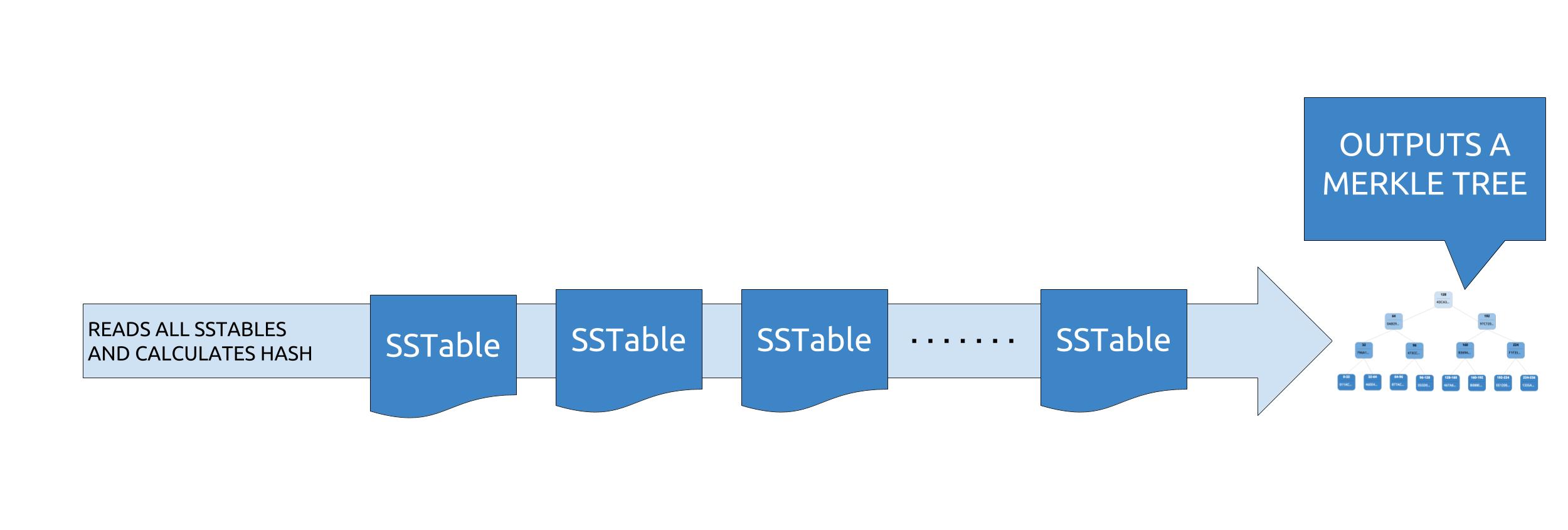
To perform repairs without comparing all data between all replicas, Apache Cassandra uses merkle trees to compare trees of hashed values instead.
During a repair, each replica will build a merkle tree, using what is called a “validation compaction”. It is basically a compaction without the write phase, the output being a tree of hashes.
Merkle trees will then be compared between replicas to identify mismatching leaves, each leaf containing several partitions. No difference check is made on a per partition basis : if one partition in a leaf is not in sync, then all partitions in the leaf are considered as not being in sync. When more data is sent over than is required it’s typically called overstreaming. Gigabytes of data can be streamed, even for one bit of difference. To mitigate overstreaming, people started performing subrange repairs by specifying the start/end tokens to repair by smaller chunks, which results in having less partitions per leaf.
With clusters growing in size and density, performing repairs within gc_grace_seconds started to get more and more challenging, with repairs sometimes lasting for tens of days. Some clever folks leveraged the immutable nature of SSTables and introduced incremental repair in Apache Cassandra 2.1.
What is incremental repair?
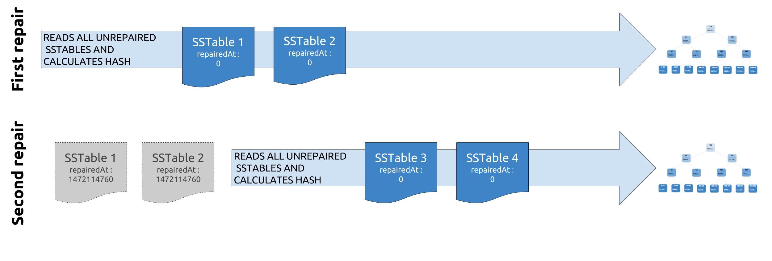
The plan with incremental repair was that once some data had been repaired, it would be marked as such and never needed to be repaired anymore.
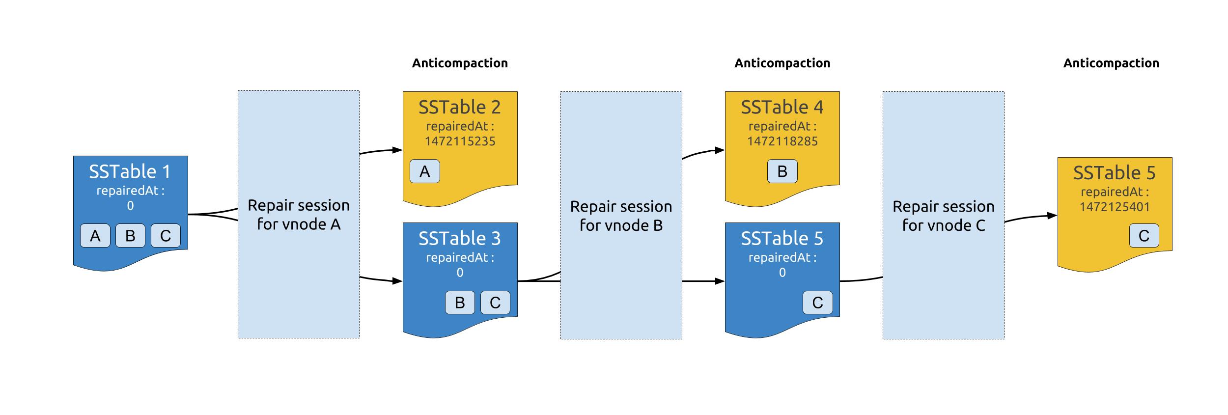
Since SSTables can contain tokens from multiple token ranges, and repair is performed by token range, it was necessary to be able to separate repaired data from unrepaired data. That process is called anticompaction.
Once a repair session ends, each repaired SSTable will be split into 2 SSTables : one that contains the data that was repaired in the session (ie : data that belonged to the repaired token range) and another one with the remaining unrepaired data. The newly created SSTable containing repaired data will be marked as such by setting its repairedAt timestamp to the time of the repair session.
When performing validation compaction during the next incremental repair, Cassandra will skip the SSTables with a repairedAt timestamp higher than 0, and thus only compare data that is unrepaired.
We currently send an anticompaction request to all replicas. During this, a node will split stables and mark the appropriate ones repaired.
The problem is that this could fail on some replicas due to many reasons leading to problems in the next repair.
This is what I am suggesting to improve it.
1) Send anticompaction request to all replicas. This can be done at session level.
2) During anticompaction, stables are split but not marked repaired.
3) When we get positive ack from all replicas, coordinator will send another message called markRepaired.
4) On getting this message, replicas will mark the appropriate stables as repaired.
This will reduce the window of failure. We can also think of "hinting" markRepaired message if required.
Also the stables which are streaming can be marked as repaired like it is done now.
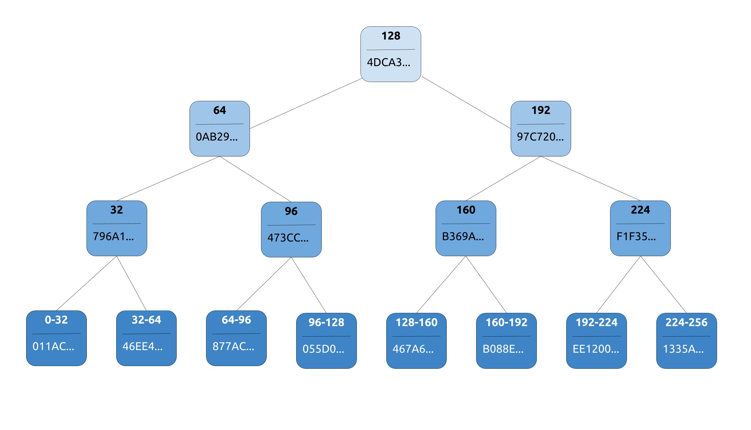
Cassandra's AntiEntropy service uses Merkle trees to detect the inconsistencies in data between replicas. Merkle tree is a hash tree where leaves contain hashes of individual data blocks and parent nodes contain hashes of their respective children. It provides an efficient way to find differences in data blocks stored on replicas and reduces the amount of data transferred to compare the data blocks.
Cassandra's implementation of Merkle tree (org.apache.cassandra.utils.MerkleTree) uses perfect binary tree where each leaf contains the hash of a row value and each parent node contains hash of its right and left child. In a perfect binary tree all the leaves are at the same level or at same depth. A perfect binary tree of depth h contains 2^h leaves. In other terms if a range contains n tokens then the Merkle tree representing it contains log(n) levels.
When nodetool repair command is executed, the target node specified with -h option in the command, coordinates the repair of each column family in each keyspace. A repair coordinator node requests Merkle tree from each replica for a specific token range to compare them. Each replica builds a Merkle tree by scanning the data stored locally in the requested token range. The repair coordinator node compares the Merkle trees and finds all the sub token ranges that differ between the replicas and repairs data in those ranges.
A replica node builds a Merkle tree for each column family to represent hashes of rows in a given token range. A token range can contain up to 2^127 tokens when RandomPartitioner is used. Merkle tree of depth 127 is required which contains 2^127 leaves. Cassandra builds a compact version of Merkle tree of depth 15 to reduce the memory usage to store the tree and to minimize the amount of data required to transfer Merkle tree to another node. It expands the tree until a given token range is split in to 32768 sub ranges. In the compact version of tree, each leaf represents hash of all rows in its respective sub range. Regardless of their size and split, two Merkle trees can be compared if they have same hash depth.
For example, the token range (0, 256], contains 256 sub ranges (0, 1], (1, 2]...(255, 256] each containing single token. A perfect binary tree of depth 8 is required to store all 256 sub range hashes at leaves. A compact version of tree with depth 3 for the same range contains only 8 leaves representing hashes of sub ranges (0, 32], (32, 64] ... (224, 256] each containing 32 tokens. Each leaf hash in this compact version of tree is a computed hash of all the nodes under it in the perfect binary tree of depth 8.
Building Merkle tree with RandomPartitioner
RandomPartitioner distributes keys uniformly , so the Merkle tree is constructed recursively by splitting the given token range in to two equal sub ranges until maximum number of sub ranges are reached. A root node is added with the given token range (left, right] and the range is split in to two halves at a token which is at the midpoint of the range. A left child node is added with range (left, midpoint] and a right child node is added with range covering (midpoint, right]. The process is repeated until required number of leaves (sub ranges) added to the tree.
Next row hashes are added to the Merkle tree in sorted order. Each row's hash value is computed by calculating MD5 digest of row value which includes row's column count, column names and column values but not the row key and row size. The deleted rows (tombstones) hashes are also added to the tree which include the delete timestamps. Row hashes are added to Merkle tree leaves based on their tokens. If a leaf's sub range contains multiple rows, its hash is computed by combining hashes of all rows covered by its range using XOR operation. Non leaf nodes hashes are computed by performing XOR on hashes of their respective children.
Comparing Merkle trees
Two Merkle trees are compared if both of them cover the same token range regardless of their size. The trees are compared recursively starting at root hash. If root hashes match in both the trees then all the data blocks in the tree's token range are consistent between replicas. If root hashes disagree, then the left child hashes are compared followed next by right child hashes. The comparison proceeds until all the token ranges that differ between the two trees are calculated.
Rapid read protection allows Cassandra to still deliver read requests when the original selected replica nodes are down or taking too long to respond.
The table needs to be configured with the speculative_retry property. The coordinator node for the read request will retry the request with another replica if the original replica node is unable to respond in the configured time.
The rapid read protection will be useful when one of the replicas is overloaded and unable to respond. If the complete cluster is already overloaded then this kind of protection guarantee can increase the number of requests and further amplify the load on Cassandra.
@Override
public String getKeyspaceName() {
return "example";
}
@Bean
public CassandraTemplate cassandraTemplate(Session session) {
return new CassandraTemplate(session);
}
@Override
public String[] getEntityBasePackages() {
return new String[] { User.class.getPackage().getName() };
}
@Override
public SchemaAction getSchemaAction() {
return SchemaAction.RECREATE;
}
}
@EnableCassandraRepositories
@Data
@NoArgsConstructor
@Table(value = "users")
public class User { @PrimaryKey("user_id") private Long id; @Column("uname") private String username; @Column("fname") private String firstname; @Column("lname") private String lastname;
public User(Long id) { this.setId(id); }
}
public interface BasicUserRepository extends CrudRepository<User, Long> {
@Query("SELECT * from users where user_id in(?0)") User findUserByIdIn(long id);
* Derived query method. This query corresponds with {@code SELECT * FROM users WHERE uname = ?0}.
* {@link User#username} is not part of the primary so it requires a secondary index.
User findUserByUsername(String username); List<User> findUsersByLastnameStartsWith(String lastnamePrefix);
} http://www.datastax.com/dev/blog/new-in-cassandra-3-0-materialized-views Materialized views handle automated server-side denormalization, removing the need for client side handling of this denormalization and ensuring eventual consistency between the base and view data. This denormalization allows for very fast lookups of data in each view using the normal Cassandra read path.
The base replica performs a local read of the data in order to create the correct update for the view. If the primary key of the view has been updated in the base table, a tombstone would need to be generated so that the old value is no longer present in the view. The batchlog is used to provide an equivalent eventual consistency to what is provided on the base table. Without the batchlog if view updates are not applied but the base updates are, the view and the base will be inconsistent with each other. Using the batchlog, however, does add significant overhead, especially since the batchlog must be written to twice.
If the rows are to be combined before placed in the view, materialized views will not work. Materialized views will create a CQL Row in the view for each CQL Row in the base
In Cassandra, two types of columns have a special role: the partition key columns and the clustering columns. Together, they will define your row primary key.
The partition key columns are the first part of primary key and their role is to spread data evenly around the cluster. Rows will be spread around the cluster based on the hash of the partition keys.
The clustering key columns are used to cluster the data of a partition, allowing a very efficient retrival of rows.
Partition keys restrictions
The partition key columns support only two operators: = and IN
IN restriction
Prior to 2.2, the IN restrictions could only be applied to the last column of the partition key
In 2.1, you could only use an IN operator on the date column. In 2.2 you can use the IN operator on any partition key column.
CREATETABLEnumberOfRequests (
cluster text,
datetext,
timetext,
numberOfRequests int,
PRIMARYKEY((cluster, date), time)
)
Unrestricted partition key columns
Cassandra will require that you either restrict all the partition key columns, or none of them unless the query can use a secondary index.
will be rejected as the date column is not restricted.
The reason why is that Cassandra needs all the partition key columns to be able to compute the hash that will allow it to locate the nodes containing the partition.
If no restrictions are specified on the partition keys but some are specified on the clustering keys, Cassandra will require ALLOW FILTERING to be added to the query.
Direct queries on secondary indices support only =, CONTAINS or CONTAINS KEY restrictions.
The CONTAINS restriction can only be used on collection types. The CONTAINS KEY restriction can only be used on map for which the keys have been indexed.
For example, if you have the following table:
1
2
3
4
5
6
7
8
9
10
CREATETABLEcontacts (
id intPRIMARYKEY,
firstName text,
lastName text,
phones map<text, text>,
emails set<text>
);
CREATEINDEXONcontacts (firstName);
CREATEINDEXONcontacts (keys(phones)); // Using the keys functiontoindexthe map keys
When Cassandra must perform a secondary index query, it will contact all the nodes to check the part of the secondary index located on each node. If all the partition key components are restricted, Cassandra will use that information to
query only the nodes that contains the specified partition keys, which will make the query more efficient.
For secondary index queries, only = restrictions are supported on partition key columns.
https://dzone.com/articles/how-not-to-start-with-cassandra Red Flag Number One — Using Cassandra on Single Node make sure you work with at least three nodes from the beginning. Problems in distributed systems are completely different from problems on single node systems, just to name a few: consuming messages exactly once, saving files to file systems, scheduling, locking. The point to take here is that you should always start developing against a truly distributed system, if you have a need for distributed technology like Cassandra, start a three node cluster from the beginning and develop against it. Red Flag Number Two — Relational World Data Modeling In Cassandra, it is important to use query based modeling, you need to know how you will read your data before modeling it. It is a distributed system, so data should be denormalized and replicated, with a lot of duplications. It is a common thing to see the same data spread across many tables, each optimized for a different read query. Red Flag Number Three — Evolving Data Model you need the best data model for each feature, so if the feature requirements are changed, the data model should be changed also. In query based modeling, the data model is exposed all the way up (this is a tradeoff to achieve performance) so it should evolve as feature requirements evolve. That was the prime reason why we came up with Cassandra Migration Tool, a supporting library which stores the database version and eases up Schema and Data changes. http://stackoverflow.com/questions/2359159/cassandra-port-usage-how-are-the-ports-used
So my complete list would be for current versions of Cassandra:
7199 - JMX (was 8080 pre Cassandra 0.8.xx)
7000 - Internode communication (not used if TLS enabled)
7001 - TLS Internode communication (used if TLS enabled)
Cassandra all of its nodes are functionally equal
Clients can connect to any of Cassandra’s nodes and when they connect to one, that node becomes the client’s session coordinator. Clients do not need to know which nodes have what data, nor do they have to be aware of outages, repairing data, or replication. Clients send all of their requests to the session coordinator and the coordinator takes responsibility for all of the internal cluster activities like replication or sharding.
Clients then issue their queries to the coordinator node they chose without any knowledge about the topology or state of the cluster. Since each of the Cassandra nodes knows the status of all of the other nodes and what data they are responsible for, they can delegate queries to the correct servers. The fact that clients know very little about the topology of the cluster is a great example of decoupling and significantly reduces complexity on the application side.
Functional partitioning of the web services layer and using different data stores based on the business needs is often referred to as polyglot persistence, and it is a growing trend among web applications.
Cassandra performs data partitioning automatically so that each of the nodes gets a subset of the overall data set. None of the servers needs to have all of the data, and Cassandra nodes communicate among one other to make sure they all know where parts of the data live.
The Cassandra data model is based on a wide column, similar to Google’s BigTable. In a wide column model, you create tables and then each table can have an unlimited number of rows. Unlike the relational model, tables are not connected, each table lives independently, and Cassandra does not enforce any relationships between tables or rows.
Cassandra tables are also defined in a different way than in relational databases. Different rows may have different columns (fields), and they may live on different servers in the cluster. Rather than defining the schema up front, you dynamically create fields as they are required. This lack of upfront schema design can be a significant advantage, as you can make application changes more rapidly without the need to execute expensive alter table commands any time you want to persist a new type of information.
The flip side of Cassandra’s data model simplicity is that you have fewer tools at your disposal when it comes to searching for data. To access data in any of the columns, you need to know which row are you looking for, and to locate the row, you need to know its row key (something like a primary key in a relational database).
When you send your query to your session coordinator, it hashes the row key (which you provided) to a number. Then, based on the number, it can find the partition range that your row key belongs to (the correct shard). Finally, the coordinator looks up which Cassandra server is responsible for that particular partition range and delegates the query to the correct server.
you can specify how many copies of each piece of data you want to keep across the cluster, and session coordinators are responsible for ensuring the correct number of replicas.
how well automated it is and how little administration it requires. For example, replacing a failed node does not require complex backup recovery and replication offset tweaking.
All you need to do to replace a broken server is add a new (blank) one and tell Cassandra which IP address this new node is replacing. All of the data transferring and consistency checking happens automatically in the background. Since each piece of data is stored on multiple servers, the cluster is fully operational throughout the server replacement procedure. Clients can read and write any data they wish even when one server is broken or being replaced. As soon as node recovery is finished, the new node begins processing requests and the cluster goes back to its original capacity.
From a scalability point of view, Cassandra is a truly horizontally scalable data store. The more servers you add, the more read and write capacity you get, and you can easily scale in and out depending on your needs.Since data is sliced into a high number of small partition ranges, Cassandra can distribute data more evenly across the cluster. In addition, since all of the topology is hidden from the clients, Cassandra is free to move data around. As a result, adding new servers is as easy as starting up a new node and telling it to join the cluster. Again, Cassandra takes care of rebalancing the cluster and making sure that the new server gets a fair share of the data.
Cassandra loves writes deletes are the most expensive type of operation you can perform in Cassandra.
Cassandra uses append-only data structures, which allows it to write inserts with astonishing efficiency. Data is never overwritten in place and hard disks never have to perform random write operations, greatly increasing write throughput. But that feature, together with the fact that Cassandra is an eventually consistent data store, forces deletes and updates to be internally persisted as inserts as well. As a result, some use cases that add and delete a lot of data can become inefficient because deletes increase the data size rather than reducing it (until the compaction process cleans them up).
http://prismoskills.appspot.com/lessons/Cassandra/Chapter_1_-_Cassandra_Introduction.jsp
Massively scalable
Linearly scalable (If 2 nodes handle x traffic, then 4 nodes handle 2x!)
NoSQL Database
Failed nodes can be replaced with no downtime.
Integrates with Hadoop and has MapReduce support. Also supports Apache Pig and Hive.
Can store structured and unstructured data alike.
Architecture Masterless architecture - meaning all nodes are the same. Data automatically distributed among all nodes in the ring. Replication factor is configurable. Replication can be configured to work across data-centers also. Failed nodes' data is automatically replicated to maintain replication factor. Cassandra emphasizes denormalization.
Language Features (CQL 3.0)
CQL has drivers available in Java, Python and Node.JS
Does not support joins or subqueries, except for batch analysis through Hive.
Lightweight transactions using the IF keyword in INSERT and UPDATE statements.
Initial support for triggers.
Data Model Cassandra is essentially a hybrid between a key-value and a column-oriented (or tabular) database.
Cassandra's column-family resembles a Table in RDBMS.
Column families contain rows and columns. Each row has multiple columns, each of which has a name, value, and a timestamp. Different rows in the same column family do not have to share the same set of columns. Columns may be added to one or multiple rows at any time.
Each key in Cassandra identifies one row with multiple columns (like a Primary Key).
nodetool -h localhost info https://gigadom.wordpress.com/2011/05/13/design-principles-of-scalable-distributed-systems/
Vector Clocks
Distributed Hash Table (DHT)
Quorum Protocol Gossip Protocol
This is the most preferred protocol to allow the servers in the distributed system to become aware of server crashes or new servers joining into the system, Membership changes and failure detection are performed by propagating the changes to a set of randomly chosen neighbors, who in turn propagate to another set of neighbors. This ensures that after a certain period of time the view becomes consistent.
Hinted Handoff and Merkle trees
To handle server failures replicas are sometimes sent to a healthy node if the node to which it was destined was temporarily down. For e.g. data destined for Node A is delivered to Node D which maintains a hint in its metadata that the data is to be eventually handed off to Node A when it is healthy.
Merkle trees are used to synchronize replicas amongst nodes. Merkle trees minimize the amount of data that needs to be transferred for synchronization.
If the primary key only contains the partition key then the table has skinny rows
If the primary key contains columns other than the partition key then the table has wide rows
In CQL “wide rows” just means that there can be more than one row per partition. Thus a table with a single column primary key has skinny rows, and a table with a compound primary key can have wide or skinny rows depending on the partition key.
Another way to put it is that CQL tables with clustering columns have wide rows.
As an example, this CQL table has skinny rows because tweet_id is the only column in the primary key:
To finish it off here’s an example of a CQL table with a compound primary key, a composite partition key, and wide rows. It has wide rows because event_time is in the primary key but is not part of the partition key:
1234567
CREATE TABLE temperature_by_day (
   weatherstation_id text,
   date text,
   event_time timestamp,
   temperature text,
   PRIMARY KEY ((weatherstation_id,date),event_time)
);
If the primary key only contains the partition key then the table has skinny rows
If the primary key contains columns other than the partition key then the table has wide rows
In CQL “wide rows” just means that there can be more than one row per partition. Thus a table with a single column primary key has skinny rows, and a table with a compound primary key can have wide or skinny rows depending on the partition key.
In CQL you can have collection type columns - set, list, map
Column can contain a user defined type (you can define e.g. address as type, and reuse this type in many places), or collection can be a collection of user defined types
https://www.tutorialspoint.com/cassandra/cassandra_data_model.htm The outermost container is known as the Cluster. For failure handling, every node contains a replica, and in case of a failure, the replica takes charge. Cassandra arranges the nodes in a cluster, in a ring format, and assigns data to them.
Keyspace is the outermost container for data in Cassandra. The basic attributes of a Keyspace in Cassandra are −
Replication factor − It is the number of machines in the cluster that will receive copies of the same data.
Replica placement strategy − It is nothing but the strategy to place replicas in the ring. We have strategies such as simple strategy(rack-aware strategy), old network topology strategy (rack-aware strategy), and network topology strategy (datacenter-shared strategy).
Column families − Keyspace is a container for a list of one or more column families. A column family, in turn, is a container of a collection of rows. Each row contains ordered columns. Column families represent the structure of your data. Each keyspace has at least one and often many column families.
Relational Table
Cassandra column Family
A schema in a relational model is fixed. Once we define certain columns for a table, while inserting data, in every row all the columns must be filled at least with a null value.
In Cassandra, although the column families are defined, the columns are not. You can freely add any column to any column family at any time.
Relational tables define only columns and the user fills in the table with values.
In Cassandra, a table contains columns, or can be defined as a super column family.
A column is the basic data structure of Cassandra with three values, namely key or column name, value, and a time stamp. Given below is the structure of a column.
To answer the original question you posed: a column family and a table are the same thing.
The name "column family" was used in the older Thrift API.
If you need to use "group by,order by,count,sum,ifnull,concat ,joins and some times nested querys" as you state then you probably don't want to use Cassandra, since it doesn't support most of those.
It is very strongly recommended that you not use supercolumns, especially in new design. They have never been problem-free, and now they are deprecated and much more capably replaced by composite keys.
It is very strongly recommended that you not use supercolumns, especially in new design. They have never been problem-free, and now they are deprecated and much more capably replaced by composite keys.
Your data could be nicely represented like this in CQL 3, for example:
If you need to use "group by,order by,count,sum,ifnull,concat ,joins and some times nested querys" as you state then you probably don't want to use Cassandra, since it doesn't support most of those.
The model in Cassandra is that rows contain columns. To access the smallest unit of data (a column) you have to specify first the row name (key), then the column name.
So in a columnfamily called Fruit you could have a structure like the following example (with 2 rows), where the fruit types are the row keys, and the columns each have a name and value.
One difference from a table-based relational database is that one can omit columns (orange has no variety), or add arbitrary columns (orange has origin) at any time. You can still imagine the data above as a table, albeit a sparse one where many values might be empty.
However, a "column-oriented" model can also be used for lists and time series, where every column name is unique (and here we have just one row, but we could have thousands or millions of columns):
temperature ->  2012-09-01  2012-09-02  2012-09-03 ...
                40          41          39         ...
which is quite different from a relational model, where one would have to model the entries of a time series as rows not columns.
It perfectly explains the difference. In such way, Cassandra could be column oriented, but it depends on you use the column names.
Column based storage became popular for warehousing, because it offers extreme compression and reduced IO for full table scans (DW) but at the cost of increased IO for OLTP when you needed to pull every column (select *). Most queries don't need every column and due to compression the IO can be greatly reduced for full table scans for just a few columns. Let me provide an example
We have two different fruits, but both have a colour = red. If we store colour in a separate disk page (block) from weight, price and variety so the only thing stored is colour, then when we compress the page we can achieve extreme compression due to a lot of de-duplication. Instead of storing 100 rows (hypothetically) in a page, we can store 10,000 colour's. Now to read everything with the colour red it might be 1 IO instead of thousands of IO's which is really good for warehousing and analytics, but bad for OLTP if I need to update the entire row since the row might have hundreds of columns and a single update (or insert) could require hundreds of IO's.
https://cassandra.apache.org/doc/cql3/CQL.html#counters
The counter type is used to define counter columns. A counter column is a column whose value is a 64-bit signed integer and on which 2 operations are supported: incrementation and decrementation (see UPDATE for syntax). Note the value of a counter cannot be set. A counter doesn’t exist until first incremented/decremented, and the first incrementation/decrementation is made as if the previous value was 0. Deletion of counter columns is supported but have some limitations (see the Cassandra Wiki for more information).
The use of the counter type is limited in the following way:
It cannot be used for column that is part of the PRIMARY KEY of a table.
A table that contains a counter can only contain counters. In other words, either all the columns of a table outside the PRIMARY KEY have the counter type, or none of them have it.
Creating a global sequential sequence of number does not really make any sense in a distributed system. Use UUIDs.
(Because you would have to make all participants agree and accept the evolution of the sequence -- under a naive implementation)
CREATE TABLE ship_sightings (
  day TEXT,
  time TIMESTAMP,
  ship TEXT,
  PRIMARY KEY (day, time)
)
And you insert entries with
INSERT INTO ship_sightings (day, time, ship) VALUES ('Tuesday', NOW(), 'Titanic')
however, you should probably use a TIMEUUID instead of TIMESTAMP (and the primary key could be a DATE), since otherwise you might add two sightings with the same timestamp and only one will survive.
Each Node in cassandra is responsible for range of hash value of partition key (Consistent hashing).
By default casssandra uses MurMur3 partitioner.
So on each node in cassandra there will be multiple partition keys availaible. For same partition key there will be only one record on one node, other copies will be available on other nodes based on replication factor.Consistent Hashing in cassandra


skinnyorwide